
|
In a blank Excel worksheet, add the text and values shown -- except in B7, enter a formula to compute the sum of the cells B3, B4, and B5.
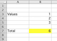
B7:"=SUM(B3:B5)"
In a blank Excel worksheet, add the text and values shown -- except in B7, enter a formula to compute the average of all the values in the other cells.
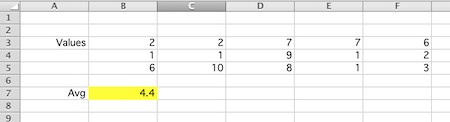
B7:"=AVERAGE(B3:F5)"
In a blank Excel worksheet, add the text in A1. Then type the contents of no more than 4 cells into their respective locations, using autofill to duplicate the rest of the worksheet shown.
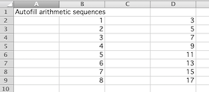
Fill B2 and B3 as shown, then select these two and autofill down to B9 (i.e., click and drag the small blue square in the bottom right corner of the selection until B2:B9 is selected, and then release the mouse button.) Do the same for the second sequence -- type in the values for cells D2:D3, select these two cells, and then autofill down to D9.
The first two terms of the Fibonacci sequence are both 1, with every other term found by summing the two terms before it. In a blank Excel worksheet, add the text seen in the cells below with white backgrounds. Then, enter a formula in B4 that can be copied or autofilled down to B11 to produce the first ten terms of the Fibonacci sequence, as shown.
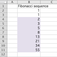
B4 : "=B2+B3"
In a blank worksheet, use autofill to generate the numbers shown with a white background. Then enter a single formula in C3 and copy it to the rest of the pink cells to create the multiplication table shown.
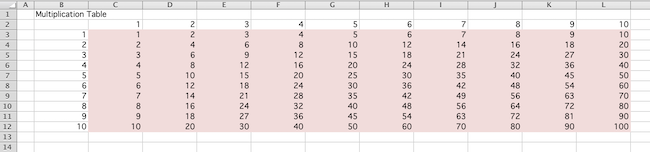
C3 : "=C$2*$B3"
In statistics, one often has to calculate the $z$-score for a particular data value $x$, in accordance with the following formula:
$$z = \frac{x - \mu}{\sigma}$$ where $\mu$ (mu) and $\sigma$ (sigma) are the mean and standard deviation of the related population.Type the data values seen in the column E into a blank Excel worksheet.
Add the labels seen in cells B2, B3, E1, and F1, and the value for $\mu$ and $\sigma$ in cells C2 and C3 as shown.
Then, type a single Excel formula into cell F2 that can be copied to F3:F11 so that the $z$-value for each data value $x$ appears to the $x$-value's immediate right.
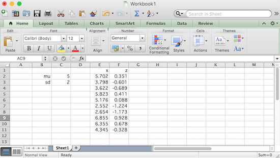
F2:"=(E2-$C$2)/$C$3"
Create a worksheet in Excel that displays a list of the first $10$ squares, like the one shown below, by entering a 1 in cell B2 and a formula in B3 that when copied to cells B4:B11 produces the desired result. (Hint: you will likely want to use the SQRT() function, which returns the square root of its argument.)
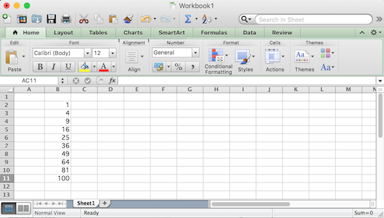
B3:"=(SQRT(B2)+1)^2"
Reproduce the contents of the cells with a white background in a blank Excel worksheet, then use formulas in the two colored cells to answer the questions posed. Note, for the second question, if any of the values in F6:I6 are changed, the answer seen in F8 should automatically update itself accordingly.
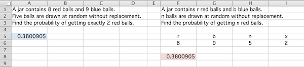
A5 : "=COMBIN(8,2)*COMBIN(9,3)/COMBIN(17,5)"
F8 : "=COMBIN(F6,I6)*COMBIN(G6,H6-I6)/COMBIN(F6+G6,H6)"
In statistics, the variance of a sample, $s^2$, can be found in two equivalent ways. If the sample consists of values $x_1, x_2, \ldots, x_{10}$ and $n$ is the size of the sample ($n=10$, in this case), and $\overline{x}$ (pronounced "x-bar") is the average of the sample values, then the variance of the sample can be calculated in accordance with either of the following expressions
$$s^2 = \frac{\sum_{i=1}^n (x_i - \overline{x})^2}{n-1} \quad \quad \textrm{ or } \quad \quad s^2 = \frac{n \sum_{i=1}^n x_i^2 - \left( \sum_{i=1}^n x_i \right)^2}{n(n-1)}$$Fill B3:B12 with the values shown below. Then, add the column and cell labels in B2, C2, D2, F2, F3, F5, and F6, as shown.
Use appropriate formulas and autofill to calculate the squared $x$'s in column C, and the squared differences between each $x$ and $\overline{x}$ in column D.
Finally, add formulas to cells G2, G3, G5, and G6 to calculate the values described by the labels to their left, where the sample variance calculations 1 and 2 refer to the formulas given above, respectively. If everything goes well, you should see cells G5 and G6 agree in value. (Hint: you may find the COUNT() function useful.)
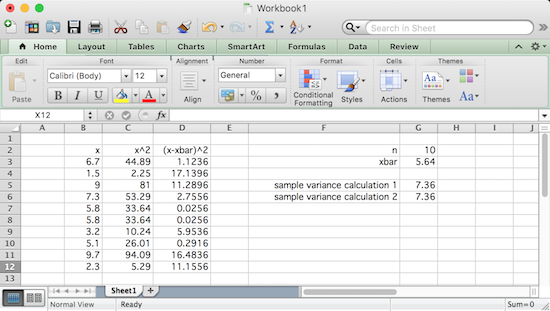
C3:"=B3^2"                    # then autofill or copy and paste down to C12
D3:"=(B3-$G$3)^2"             # then autofill or copy and paste down to D12
G2:"=COUNT(B3:B12)"
G3:"=AVERAGE(B3:B12)"
G5:"=SUM(D3:D12)/(G2-1)"
G6:"=(G2*SUM(C3:C12)-SUM(B3:B12)^2)/(G2*(G2-1))"
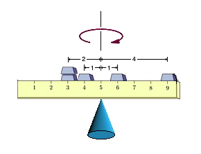
Imagine several lead weights of equal mass are glued at different positions along the top of a ruler. Assuming the ruler has a negligible mass and width, the whole thing is balanced on a small triangular prism that functions as a fulcrum, as shown in the picture below.
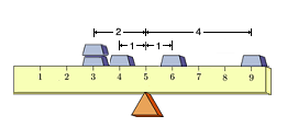
If the masses are to balance atop the triangular prism without tipping to one side or the other, the collective torque of the masses to the left of the triangular prism must be equal in magnitude to the collective torque of the masses to the right of the triangle, but be opposite in direction (i.e., sign).
For those that have not encountered torque before -- torque is the product of the force on an object and the distance to the pivot point (i.e., the triangular prism).
In the picture above, there are 5 masses. Assuming the same unit force downward on each mass, and negative torques causing the ruler to tip downwards on the left, while positive torques cause the ruler to tip downwards to the right -- if the triangular prism is placed as shown, then the 5 masses contribute torques of: $$-2,-2,-1,1,\textrm{ and } 4$$ These sum to a net torque of zero, suggesting the ruler and its weights will balance on a triangular prism that has been placed directly below the tickmark "5" on the ruler.
At any other point there will be a net positive or negative torque and the ruler will tip to one side. For example, if one placed the fulcrum at 6, then the individual torques contributed by the lead weights would be $-3, -3, -2, 0, 3$ which sum to $-5$, suggesting the left side of the ruler will move downwards.
A natural question to ask is "For a given collection of weights at various positions on the ruler, how do I find this point where everything balances?" By the way, this point is called the center of mass for the system (assuming gravitational forces are constant -- but I digress).
Here's a way we might have figured out that the center of mass of the above system was at the tickmark "5" on the ruler:
Suppose that $n$ masses are placed at positions $x_1, x_2, \ldots, x_n$ on the ruler and the center of mass is at some unknown $\mu$ on the ruler.
Assuming again that each mass experiences a unit force downward, the torque associated with a mass at position $x_i$ on the ruler is then given by $(x_i - \mu)$.
Conveniently, when the mass is to the left of $\mu$, note this difference is negative -- and when it is to the right of $\mu$, the difference is positive, just as in the example worked above.
When balanced, the sum of all the individual torques is zero, so $$(x_1 - \mu) + (x_2 - \mu) + \cdots + (x_n - \mu) = 0$$ Collecting like terms, we have $$(x_1 + x_2 + \cdots + x_n) - n\mu= 0$$ Solving for $\mu$, we find $$\mu = \frac{x_1 + x_2 + \cdots + x_n}{n}$$ As such, the position of the center of mass for this collection of individual masses is simply the average of their respective individual positions.
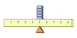
Notably, this center of mass is the one point, whereupon having already balanced the ruler, all of the individual masses could be collected together at one point and the ruler would remain balanced, as shown below.
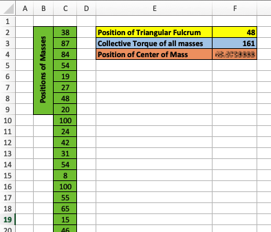
With all of this as preface, download torque.xlsx, an Excel worksheet that specifies positions of 150 equal sized masses along a 100-inch long measuring stick (of negligible mass and width). Add formulas to the necessary cells so that two things happen:
When a user enters a position for the triangular prism in cell $F2$, which is possibly a position where things are unbalanced, the collective torque of all the masses is displayed in cell $F3$. When this torque is negative, the measuring stick should tip downwards on the left -- when positive, it should tip downwards on the right.
The position the triangular prism should be placed to achieve balance (i.e., the center of mass) should be calculated in cell $F4$. Notably, if one enters this position in $F2$, the collective torque should be essentially zero (although it might be slightly off due to internal rounding errors in Excel).
To check your work, when the triangular fulcrum is placed at the tickmark for "48", the collective torque computed is 161, as shown in the worksheet below (note, the center of mass has been purposefully blurred, given a question that is about to be asked):
Use your sheet to find the following two values:
What is the sum of these two values, rounded to the nearest integer?
Answers vary, but here is one way:
F2: "52"
F3: "=SUM(C2:C151)-COUNTA(C2:C151)*F2"
F4: "=AVERAGE(C2:C151)"

Then, find the sum of these two values with "=SUM(F3:F4)",
and don't forget to round to the nearest integer (i.e., -390)
You have probably seen figure skaters spinning in place increase or decrease their speed by either drawing their arms and legs inwards, or extending them outwards, respectively.

The physics of this involves the so-called "conservation of angular momentum". Essentially, this means that with no external force to act on it, the original angular momentum of a system (like the figure skater) remains constant.
For the curious, angular momentum is the product of the system's angular velocity (measured in radians per second, for example) and the system's moment of inertia.
$$\textrm{Angular momentum } = (\textrm{Moment of Inertia}) \times (\textrm{Angular Velocity})$$The moment of inertia, in turn, of a single particle of mass $m$ rotating about some point is given by $mr^2$, where $r$ is the distance from the particle to the center of rotation.
Further -- when more particles are involved -- the moment of inertia is additive in the following sense: Suppose a body consists of $n$ particles with masses $m_1,m_2,\ldots,m_n$ at distances $r_1,r_2,\ldots,r_n$ from the center of rotation. The moment of inertia is then given by $$I = m_1r_1^2 + m_2r_2^2 + \cdots + m_nr_n^2$$ Suppose we have a collection of unit masses atop a ruler of negligible mass and width, balanced on the tip of a cone positioned at the center of mass this time so that it can spin freely. Then, start it spinning at a given angular velocity, $v_0$.
If we push all of the masses outwards, away from the center of balance and top of the cone, certainly the velocity should decrease. If we draw all of the masses inwards, the velocity increases. One might be curious if there is a single distance from the center of rotation where we could move all of the masses (half on one side, half on the other, so that it remains balanced), so that the angular velocity remains unchanged. Note, some of the masses would likely be drawn inwards, while others would be pushed outwards.
As it turns out, this distance is easy to calculate -- as if the velocity is unchanged and the angular momentum must be conserved (i.e., unchanged), then the moment of inertia, $I$, must also be unchanged.
Recalling all of the masses are unit masses (i.e., each $m_i = 1$), then for the distance we seek (let's call it $\sigma)$, the following must be true:
$$n\sigma^2 = r_1^2 + r_2^2 + \cdots + r_n^2$$ Solving for $\sigma$, we have $$\sigma = \sqrt{\frac{r_1^2 + r_2^2 + \cdots r_n^2}{n}}$$ Recalling that each $r_i$ is the distance from a mass at position $x_i$ to the center of rotation -- which in this case is the center of mass, $\mu$, described in the previous problem -- we can write this another way: $$\sigma = \sqrt{\frac{(x_1 - \mu)^2 + (x_2 - \mu)^2 + \cdots (x_n - \mu)^2}{n}}$$Note, by its construction, the distance $\sigma$ gives us an indication of how "spread out" our unit masses are. Larger $\sigma$ values correspond to unit masses that are more spread out.
Modify the Excel worksheet inertia_sheet.xlsx to find the distance $\sigma$ described above for the 150 unit mass positions given in this worksheet, rounded to the nearest integer!
Answers vary, but here is one way:
F4: "Mu"
F5: "=AVERAGE(C4:C153)"
D4: "=(C4-$F$5)^2"  and then copy and paste this to D5:D153
F7: "Sigma"
F8: "=SQRT(SUM(D4:D153)/COUNTA(D4:D153))"

Then don't forget to round down the value in F8
to the nearest integer. (i.e., 28)
Alternatively, if you read the notes on Standard Deviation and Moment of Inertia and searched a bit online for Excel functions that deal with standard deviation and rounding, you might have done this more simply with the following:
E4: "=ROUND(STDEV.P(C4:C153),0)"
★ As the (likely apocryphal) story goes, Carl Friedrich Gauss, one of the greatest mathematicians of all time, when in primary school was asked to sum the numbers from 1 to 100 by his instructor. Presumably, the instructor thought that this task would occupy his students for a while. However, after only a few seconds of thought, young Gauss realized that he could quickly find the sum of the following paired-off values:
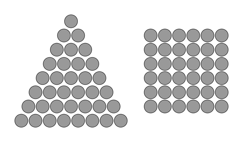
$$(1+100) + (2+99) + (3+98) + \cdots + (100+1)$$ These $100$ sums of $101$ add to twice what he was assigned to find, meaning the answer is: $$\frac{100 \cdot 101}{2} = 5050$$ This technique easily generalizes, allowing one to show: $$1 + 2 + 3 + \cdots + n = \frac{n(n+1)}{2}$$ Note that one could represent each such number using dots arranged in the shape of a triangle. The first six of these, denoted, $T_n$ are shown below.
Further, there are some numbers, like 36, that when expressed as a collection of dots can form either a triangle or a square!
As a quick-and-dirty means to test if something is a perfect square, note that when one takes a square root of a non-perfect square, the result has many digits past the decimal point. Of course the $SQRT()$ function can be used in Excel to take square roots.
Use Excel to find the largest positive integer less than 2 million that can similarly be expressed as both a triangle of dots and a square of dots.
Answers vary, but noticing that the largest value of $n$ that need be considered is the solution to $n(n+1)/2 = 2000000$, which is somewhere around $n=2000$, here is one way:
B3: "1"
B4: "=B3+1"         then copy this formula, use GoTo to quickly
                    select B5:B2005, and paste into this range

C3: "=B3*(B3+1)/2"  then similarly copy and paste this formula
                    (again using GoTo) to C5:C2005

D3: "=SQRT(C3)"     then similarly copy and paste this formula
                    (again using GoTo) to D5:D2005
Scanning column D, we see "triangular-square" numbers at $n=1,8,49,288,\textrm{ and } 1681$. Finding the value of $n(n+1)/2$ for the largest of these gives $1413721$.
Looking at the bottom of column C, we see that $n(n+1)/2$ exceeds 2 million exactly when $n = 2000$. So it must be the case that $1413721$ is the value we seek.
Perhaps more familiarly, it is the triangle of numbers that starts with a single $1$ at its top, has $1$'s down its two sides, and whose interior values are the sum of the interior values directly above them.
One can easily create a representation of Pascal's Triangle in Excel, although the numbers grow large very quickly, even after a moderate number of rows.
However, if we reduce the size of the numbers in the triangle to their remainders upon division by some constant value (called the modulus), not only do the values that result fit easily in the cells due to their smaller size -- but also, interesting patterns are revealed. Importantly, the formula "=MOD(a,b)" in Excel gives the remainder of $a$ upon division by $b$.
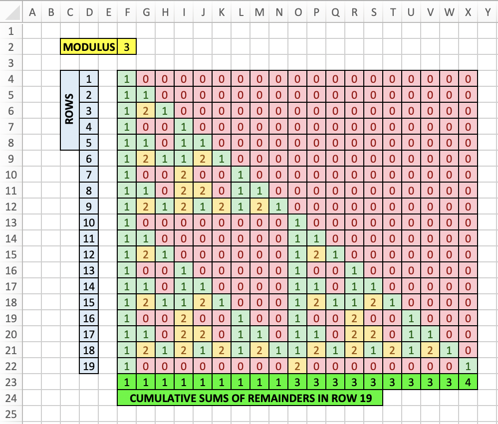
Create an Excel worksheet that looks similar to the one shown below. The values in $D4:D22$ should be consecutive integers indicating the various rows found. The top row should consist of a single $1$ in $F4$ and zeroes to its right. The range $F4:F22$ should consist of only ones.
Each value found in $G5:X22$ is determined in the following way:
First, find the sum of the values in the cells directly above and directly above and to the left of the cell in question. Then, find the remainder of this value upon division by the modulus (which the user supplies in $F2$) .
The cells can be colored automatically (as shown above) using conditional formatting. This can better highlight the interesting patterns that result for some values of the modulus -- but is not necessary for the task at hand.
Suppose one is interested in investigating the sums of the remainders that make up each row. Perhaps one seeks a pattern or formula to generate these. To this end, note that cumulative sums of the remainders shown in row 22 of the worksheet (i.e., row 19 of the triangle) are calculated in the bright green cells of row 23.
Use Excel to answer the following question: If the triangle is extended until it has 99 rows, what is the product of the last 5 cumulative sums for row 99 (i.e., the sums in columns $CV$ to $CZ$)?
To the extent it helps, the product of the last 5 cumulative sums for row 19 shown above is 324.
Answers vary, but here is one way:
D4: "1"
D5: "2"  then select D4:D5 and auto-fill down to D102

F2: "3"
F4: "1"  then select this cell and auto-fill down to F102

G4: "=MOD(SUM(F2:G2),$F$2)" then copy this cell,
                            select G4:CZ102 with GoTo and paste

F103: "=SUM($F102:CJ102)" then select this cell and
                              auto-fill to CZ103

Finally, use:
"=PRODUCT(CV103:CZ103)"
in any empty cell to find the value sought (i.e., 286925184)