
|
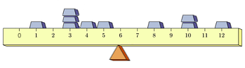
The expected value of a random variable provides a "center" for the related probability distribution seen in its probability mass function, just like the center of mass provides a "center" for a collection of masses fixed atop a ruler, at which the ruler can be balanced upon some small support, as shown:
However, just as there are multiple different arrangements of masses atop a ruler that will all balance at the same point -- there are multiple different random variables with the same expected value.
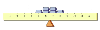
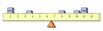
One way in which these may differ lies in how "spread out" their respective distributions are, as suggested by the two distributions of masses shown below. Both balance at 6.5, but the second is clearly far more "spread out" than the first:
Understanding that sometimes these differences in spread are harder to see than others, we seek a quantitative measure of the spread of a distribution.
As it happens, the physics of masses comes to our rescue again. You have undoubtedly seen figure skaters spinning in place increase or decrease their rotational velocity by either drawing their arms or legs inwards, or extending them outwards, respectively.

So the rotational velocity of the skater is tied to how "spread out" the distribution of mass in her body is about the center of rotation.
The reason the rotational velocity of the skater changes in this way involves the "conservation of angular momentum". Essentially, this means that with no external force to act on it, the original angular momentum of a system (like the figure skater) remains constant.
Physics tells us that angular momentum is the product of the system's angular velocity (measured in radians per second, for example) and the system's moment of inertia.
$$\textrm{Angular momentum } = (\textrm{Moment of Inertia}) \times (\textrm{Angular Velocity})$$The moment of inertia, in turn, of a single particle of mass $m$ rotating about some point is given by $mr^2$, where $r$ is the distance from the particle to the center of rotation.
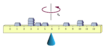
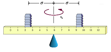
Further -- when more particles are involved -- the moment of inertia is additive in the following sense: Suppose a body consists of $n$ particles with masses $m_1,m_2,\ldots,m_n$ at distances $r_1,r_2,\ldots,r_n$ from the center of rotation. The moment of inertia is then given by $$I = m_1r_1^2 + m_2r_2^2 + \cdots + m_nr_n^2$$ Let us consider again the collection of masses atop a ruler of negligible mass and width shown at the top of this page. This time, let us balance the ruler on the tip of a cone (again positioned at the center of mass) so that it can spin freely, as shown below.
As we did when showing the connection between the expected value of a random variable and the center of mass -- while one could envision the below as 10 equal-sized masses, with three of these at position 3 on the ruler and two of these at position 10, let us again see this instead as 7 masses: five masses of size $m$ at positions 1, 4, 5, 8, and 12; a mass double that size (i.e., $2m$) at position 10; and another mass triple that size (i.e., $3m$) at position 3. This will allow us to define a more general measure of the spread of a distribution.
Now, start the system of masses spinning at some angular velocity, $v_0$.
If while the ruler is spinning, we push all of the masses outwards (away from the center of mass, where the top of the cone is located), the velocity should decrease -- just as was observed with the skater. If we draw all of the masses inwards, the velocity should correspondingly increase.
One might be curious as to whether there is a single distance (let's call it $\sigma$) from the center of rotation where we could consolidate all of the mass leaving the angular velocity unchanged (half on one side, half on the other, so that the center of mass does not change). Note, some of the masses might be drawn inwards, while others would be pushed outwards.
This $\sigma$ could then serve as a measure of the spread of this distribution of masses. It would clearly be greater as the masses started farther from the center of mass, and smaller when they started closer to the center. As it turns out, $\sigma$ is easy to calculate...
As we did when we showed the relationship between expected value and the center of mass, let us define a function $f(x)$ that for any position $x$ on the ruler, outputs the fraction of the total mass located at that position.
Again, this function $f(x)$ can easily be described by a table, as shown below
$$\begin{array}{|r|c|c|c|c|c|c|c|}\hline x & 1 & 3 & 4 & 5 & 8 & 10 & 12\\\hline f(x) & 0.1 & 0.3 & 0.1 & 0.1 & 0.1 & 0.2 & 0.1\\\hline \end{array}$$If $M$ represents the total mass, then the mass at position $x_i$ is given by $m_i = M \cdot f(x_i)$.
Recall the velocity is unchanged and the angular momentum must be conserved (i.e., unchanged), so the moment of inertia, $I$, must also be unchanged.
As such, the following must be true of $\sigma$:
$$M \sigma^2 = m_1 r_1^2 + m_2 r_2^2 + \cdots + m_n r_n^2$$ Replacing each $m_i$ with $f(x_i) \cdot M$, and each distance $r_i$ with $(x_i - \mu)$, where $\mu$ is the center of mass (i.e., where the tip of the cone and the center of rotation is located), we have $$M \sigma^2 = [M \cdot f(x_1)] (x_1 - \mu)^2 + [M \cdot f(x_2)] (x_2 - \mu)^2 + \cdots + [M \cdot f(x_n)] (x_n - \mu)^2$$ Dividing both sides by $M$ we find $$\sigma^2 = f(x_1)(x_1 - \mu)^2 + f(x_2)(x_2 - \mu)^2 + \cdots + f(x_n)(x_n - \mu)^2$$ Presuming $S$ is the set of all positions where there are masses (i.e., $S = \{x_1, x_2, \ldots, x_n\}$, We can write this in an even tighter way: $$\sigma^2 = \sum_{x \in S} (x - \mu)^2 \cdot f(x)$$ Finally, solving for $\sigma$, we have $$\sigma = \sqrt{\sum_{x \in S} (x - \mu)^2 \cdot f(x)}$$ Just as the $\sigma$ described above measures the spread of a distribution of masses, we can define a similar value to measure the spread of a probability distribution associated with a random variable and tied to its corresponding probability mass function $P(x)$. For a given random variable $X$, we refer to this as the standard deviation of $X$, denoting it by either $SD(X)$ or $\sigma$, and calculating its value in accordance with the formula: $$SD(X) = \sqrt{\sum_{x \in S} (x - \mu)^2 \cdot P(x)}$$