
|
Suppose we wish predict the body mass of two individuals whose heights are 145 and 160 cm, respectively -- based on the following paired data:
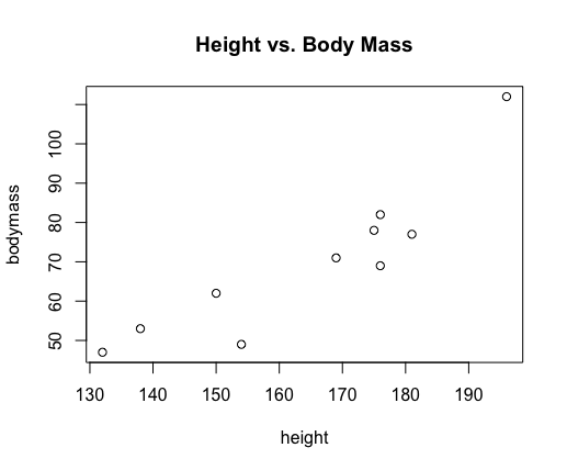
$$\begin{array}{r|c|c|c|c|c|c|c|c|c|c} \textrm{height (cm)} & 176 & 154 & 138 & 196 & 132 & 176 & 181 & 169 & 150 & 175\\\hline \textrm{body mass (kg)} & 82 & 49 & 53 & 112 & 47 & 69 & 77 & 71 & 62 & 78\\ \end{array}$$We first examine the scatter plot to make ensure the correlation, if it exists, appears to be a linear one.
> height = c(176, 154, 138, 196, 132, 176, 181, 169, 150, 175)
> bodymass = c(82, 49, 53, 112, 47, 69, 77, 71, 62, 78)
> plot(height,bodymass,main="Height vs. Body Mass")
This produces the following scatter plot:
Not seeing any issues with the scatter plot or any other assumptions of the parametric correlation test, we proceed with the test to decide if there is a significant correlation. (Recall, if no significant correlation exists, the predictions for the body mass for both heights will simply be the average body height.)
> cor.test(height,bodymass)

    Pearson's product-moment correlation

data:  height and bodymass
t = 5.8892, df = 8, p-value = 0.0003662
alternative hypothesis: true correlation is not equal to 0
95 percent confidence interval:
 0.6285267 0.9767094
sample estimates:
      cor
0.9014256
Notice, with a $p$-value of $0.0003662$ we have strong evidence that a correlation exists between height and body mass.
Now, we simply need to find the best-fit (regression) line for our data -- known as a linear model in R. We find the linear model with the lm() function:
> linear.model = lm(bodymass ~ height)
> linear.model

Call:
lm(formula = bodymass ~ height)

Coefficients:
(Intercept)       height
   -70.4627       0.8528
Importantly, notice that in the lm() function we put bodymass to the left of the tilde (~) symbol. The vector to the left of the tilde must always be the dependent variable (i.e., the one for which we wish to find predicted values), and the vector to the right of the tilde must always be the independent variable (the one on whom are predictions are based).
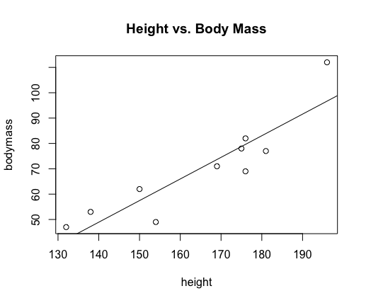
The output tells us that the best-fit (regression) line is given by $\widehat{y} = 0.8528x -70.4627$.
If one wishes to see this line added to our scatter plot, simply type the following after creating the plot:
abline(linear.model)
This adds the line stored in the variable linear.model so that our plot now looks like the following:
Now all that remains is to make our predictions by evaluating $\widehat{y}$ for $x=145$ and $x=160$.
Of course, R provides a quick way to do that too:
> linear.model$coefficients[2]*c(145,160)+linear.model$coefficients[1]
[1] 53.19906 65.99165
So our model predicts a person 145 cm tall will have body mass of around 53 kg, and a person 160 cm tall will have body mass of almost 66 kg.