
|
A population parameter is a characteristic or measure obtained by using all of the data values in a population.
A sample statistic is a characteristic or measure obtained by using data values from a sample.
The parameters and statistics with which we first concern ourselves attempt to quantify the "center" (i.e., location) and "spread" (i.e., variability) of a data set. Note, there are several different measures of center and several different measures of spread that one can use -- one must be careful to use appropriate measures given the shape of the data's distribution, the presence of extreme values, and the nature and level of the data involved.
As we consider different measures of center and spread, recall that we really want to know about the center and spread of the population in question (i.e., a parameter) -- but normally only have sample data available to us.
As such, we calculate sample statistics to estimate these population parameters.
We can characterize the shape of a data set by looking at its histogram.
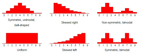
First, if the data values seem to pile up into a single "mound", we say the distribution is unimodal. If there appear to be two "mounds", we say the distribution is bimodal. If there are more than two "mounds", we say the distribution is multimodal.
Second, we focus on whether the distribution is symmetric, or if it has a longer "tail" on one side or another. In the case where there is a longer "tail", we say the distribution is skewed in the direction of the longer tail. In the case where the longer tail is associated with larger data values, we say the distribution is skewed right or (positively skewed). In the case where the longer tail is associated with smaller (or more negative) values, we say the distribution is skewed left or (negatively skewed).
If the distribution is symmetric, we will often need to check if it is roughly bell-shaped, or has a different shape. In the case of a distribution where each rectangle is roughly the same height, we say we have a uniform distribution.
The below graphic gives a few examples of the aforementioned distribution shapes.
For interval or ratio level data, one measure of center is the mean. The population mean is denoted by $\mu$, while the sample mean intended to estimate it is denoted by $\overline{x}$. Both values are calculated in a very similar way. Assuming the population has size $N$, a sample has size $n$, and $x$ spans across all available data values in the population or sample, as appropriate, we find these means by calculating $$\mu = \frac{\sum x}{N} \quad \textrm{ and } \quad \overline{x} = \frac{\sum x}{n}$$
The median, denoted by $Q_2$ (or med) is the middle value of a data set when it is written in order. In the case of an even number of data values (and thus no exact middle), it is the average of the middle two data values. It is not affected by the presence of extreme values in the data set. Unlike the mean, it can sometimes† even suggest a central value for ordinal data.
† : One can list ordinal data "in order" and find the value in the middle when there is an odd total number of values. However, when there is an even total number of values, there is a complication -- we can't average two ordinal values as we can with ratio or interval-level values to find a "middle value". As an example, suppose one's data involved ranks of poker cards: $A,7,7,10,J,Q,Q,K,K,K$. The two middle ranks are a jack (J) and a queen (Q). What would their average be? Due to the difficulty in answering this question, some texts suggest that for an even-length list of ordinal data, one should instead simply choose the lower of the two middle values to be the median.
The mode is the most frequent data value in the population or sample. There can be more than one mode, although in the case where there are no repeated data values, we say there is no mode. Modes can be used even for nominal data.
The midrange is just the average of the highest and lowest data values. While easily understood, it is strongly affected by extreme values in the data set, and does not reliably find the center of a distribution.
In addition to knowing where the center is for a given distribution, we often want to know how "spread out" the distribution is -- this gives us a measure of the variability of values taken from this distribution. The below graphic shows the general shape of three symmetric unimodal distributions with identical measures of center, but very different amounts of "spread".
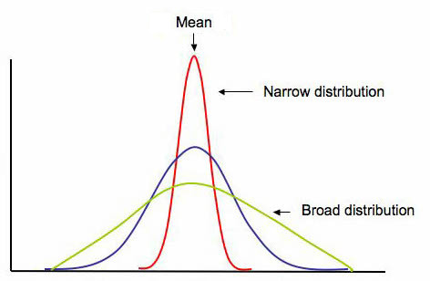
Just as there were multiple measures of center, there are multiple measures of spread -- each having some advantages in certain situations and disadvantages in others:
The range is technically the difference between the highest and lowest values of a distribution, although it is often reported by simply listing the minimum and maximum values seen. It is strongly affected by extreme values present in the distribution.
Another measure of spread is given by the mean absolute deviation, which is the average distance to the mean. Remember the distance between two values $x$ and $y$ is given by the absolute value of their difference $|x - y|$, so the distance between a value $x$ and the mean of the population $\mu$ would be $|x - \mu|$. To find the average of this distance, we sum over the population and divide by the number of things in the population, $N$: $$MAD = \frac{\sum |x - \mu|}{N}$$ While simple to express, the mean absolute deviation creates some problems for us down the line (not horribly unlike how the introduction of an absolute value inside a function -- as those that have studied calculus know -- can cause problems with regard to differentiability). Additionally, the corresponding sample statistic is a biased estimator of the population's mean absolute deviation. This means that it's average value disagrees with the populations MAD.
When the mean is the most appropriate measure of center, then the most appropriate measure of spread is the standard deviation. This measurement is obtained by taking the square root of the variance -- which is essentially the average squared distance between population values (or sample values) and the mean.
Using the square of the distances between these values and the mean gets around the difficulties introduced by the absolute value in the mean absolute deviation, although it exaggerates the contributions to the spread of the population made by values far from the mean.
On the whole, however, for our purposes, the advantages of using variance and standard deviation to measure variability and spread over the mean absolute deviation far outweigh the disadvantages.
With all this in mind, the population variance, $\sigma^2$, and population standard deviation, $\sigma$, are given by $$\sigma^2 = \frac{\sum (x-\mu)^2}{N} \quad \textrm{ and } \quad \sigma = \sqrt{\frac{\sum (x-\mu)^2}{N}}$$ When dealing with a sample, a slight alteration to the denominators in these formulas must be made in order for $s^2$ to be an unbiased estimate of the corresponding population parameter $\sigma^2$ (see Bessel's Correction), as shown below. $$s^2 = \frac{\sum (x-\overline{x})^2}{n-1} \quad \textrm{ and } \quad s = \sqrt{\frac{\sum (x-\overline{x})^2}{n-1}}$$
When the median is the most appropriate measure of center, then the interquartile range (or IQR) is the most appropriate measure of spread. When the data are sorted, the IQR is simply the range of the middle half of the data. If the data has quartiles $Q_1, Q_2, Q_3, Q_4$ (noting that $Q_2$ is the median and $Q_4$ is the maximum value), then $$IQR = Q_3 - Q_1$$ Unlike the range itself, the IQR is not easily affected by the presence of extreme data values.
Note, the presence of skewness (or outliers) can affect where the measures of center are located relative to one another, as the below graphic suggests.
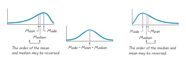
As can be seen, when significant skewness is present, the mean and median end up in different places. Turning this around, if the mean and median are far enough apart, we can determine if an observed skewness is significant.
To this end, Pearson's Skewness Index, I, is defined as $$I = \frac{3(\overline{x} - Q_2)}{s}$$ As for whether or not the mean and median are far enough apart (relative to the spread of the distribution), we say that if $|I| \ge 1$, then the data set is significantly skewed.
An outlier is a data value significantly far removed from the main body of a data set. Recall that in calculating the IQR we measure the span of the central half of a data set, from $Q_1$ to $Q_3$. It stands to reason that if a data value is too far removed from this interval, we should call it an outlier. Of course, we expect values to be farther away from the center (here, $Q_2$) when the spread (here, the IQR) is large, and closer to center when the spread is small. With this in mind, we say any value outside of the following interval is an outlier. $$[Q_1 - 1.5 \times IQR, Q_3 + 1.5 \times IQR]$$
One might wonder where the $1.5$ in the above interval comes from -- Paul Velleman, a statistician at Cornell University, was a student of John Tukey, who invented this test for outliers. He wondered the same thing. When he asked Tukey, "Why 1.5?", Tukey answered, "Because 1 is too small and 2 is too large."