
|
The number of calories contained in a selection of fast-food sandwiches is shown below: $$\begin{array}{ccccccccc} 225 & 290 & 290 & 300 & 320 & 320 & 340 & 390 & 390\\ 405 & 430 & 440 & 450 & 460 & 470 & 530 & 530 & 530\\ 535 & 540 & 560 & 580 & 610 & 660 & 675 & 730 & 1010\\ \end{array}$$
Find the mode(s) of the data
Determine if there is an outlier in the data set using a test that involves the $IQR$.
If there are at most two outliers, remove them from the data set before answering the remaining questions below
Is the distribution of data significantly skewed?
What percentage of the data lies within 2 standard deviations of the mean? Show that this result is consistent with Chebyshev's theorem
According to the Empirical Rule, for a normal distribution approximately $\underline{\hspace{1in}}$ percent of the data should lie within 2 standard deviations of the mean.
Construct a frequency distribution table for the data with 6 classes showing class limits and class boundaries. Use this to draw a frequency histogram for the data. Make sure to correctly label your graph.
Based on your answers to the previous questions, is the data set approximately normal? Explain.
530$
$Q_1 = 340$; $Q_3 = 560$; $IQR = 220$; $Q_1 - 1.5 \cdot IQR = 10$; $Q_3 + 1.5 \cdot IQR = 890$; so $1010$ is an outlier.
After removing outlier $1010$, we have $\overline{x} \doteq 461.54$; $s \doteq 132.55$; $Q_2 = 455$; so $I = 3(\overline{x}-Q_2)/s \doteq 0.1479$. Data is not significantly skewed as $-1 \lt I \lt 1$.
$\overline{x}-2s = 196.438$; $\overline{x} + 2s \doteq 726.639$; $25/26 \doteq 96.15\%$ is within 2 standard deviations of the mean. Chebyshev's theorem claims that at least $75\% = 1-1/2^2$ is within two standard deviations from the mean -- so this is consistent with the results found.
$95\%$
Limits        Boundaries        Frequency
220 - 309     219.5 - 309.5     4
310 - 399     309.5 - 399.5     5
400 - 489     399.5 - 489.5     6
490 - 579     489.5 - 579.5     6
580 - 669     579.5 - 669.5     3
670 - 759     669.5 - 759.5     2
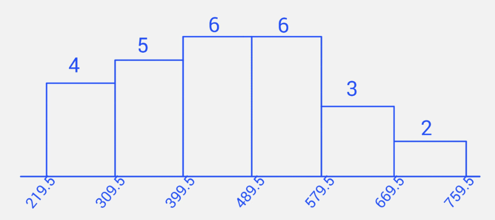
Yes. After the outlier has been removed, the data set is not significantly skewed and the histogram is approximately unimodal and symmetric.
The mean weight of an airline passenger's suitcase is $45$ pounds. Assume the weights are normally distributed and the standard deviation is 2 pounds.
Find the probability that a randomly selected suitcase weighs between 42 and 48 pounds.
Find the probability that the mean weight of 10 randomly selected suitcases is greater than 46 pounds
For a sample of 150 randomly selected suitcases, how many of them would you expect to weigh greater than 50 pounds?
At least what weight are the heaviest 10% of suitcases?
$P(42 \lt x \lt 48) = P(-1.5 \lt z \lt 1.5) = P(z \lt 1.5) - P(z \lt -1.5) = 0.8664$
CLT applies. Mean weights of samples of size 10 are normally distributed as the population of suitcase weights is normally distributed. $\mu_{\overline{x}} = 45$; $\sigma_{\overline{x}} = 2/\sqrt{10} = 0.632$; $P(\overline{x} \gt 46) = P(z \gt 1.58) = P(z \lt -1.58) = 0.0571$
$P(x \gt 50) = P(z \gt 2.5) = P(z \lt -2.5) = 0.0062$, Therefore in a group of 150 suitcases, the expected number of those who weigh more than 50 pounds is $150 \cdot 0.0062 \doteq 0.93$, or approximately 1 suitcase
First find the cutoff $z$-score that has $0.10$ area to its right, and thus $0.90$ area to its left. (On a table, look up $0.9000$ in the body of the table; on a TI-calculator, use invNorm(0.9)) This results in $z = 1.285$. Now find $x = 45 + 1.285 \cdot 2 = 47.57$. So $47.57$ pounds is the least weight for the heaviest 10% of suitcases.
Fill-in-the-blank and short answer questions:
A $\underline{\hspace{1in}}$ is a numerical measurement describing some characteristic of a population. The symbol for the variance of a population is $\underline{\hspace{1in}}$
An example of ordinal level data is $\underline{\hspace{1in}}$
Temperature (in $F^{\circ}$ is an example of $\underline{\hspace{1in}}$ level data.
According to Chebyshev's Theorem, for any distribution at least $\underline{\hspace{1in}}$ percent of the data must lie within $1.6$ standard deviations of the mean
The standard normal distribution has mean equal to $\underline{\hspace{1in}}$ and standard deviation equal to $\underline{\hspace{1in}}$.
For a normal distribution with mean 60 and standard deviation 10, approximately $\underline{\hspace{1in}}$ percent of the data lies between 50 and 70.
Describe what is meant by cluster sampling.
Divide the population in groups (or clusters), and randomly select some of these groups. Use all members from the selected groups.
Describe two problems with the sampling in the 1936 Literary Digest election poll.
It was voluntary, so only the people who are very interested responded. Also, the surveys were sent to a group that, in general, had a higher income than the general public which biased the results towards Alf Landon.
Consider the following situation: "Most foreign skiers involved in accidents in a Swiss skiing resort came from Germany". Is it correct to conclude that being German increases your chance of being in an accident at that particular skiing resort? Justify your answer.
No. We can't blame Germans for most of the accidents without knowing something about the composition of the foreign skiers. If most of the foreign skiers are German, then it expected that most of the ski accidents involve Germans, and the fact of being German has nothing to do with how likely you are to get involved in an accident at that particular ski resort.