
|
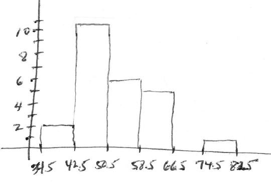
Consider the following data set: $$\begin{array}{ccccc} 35 & 39 & 43 & 43 & 43\\ 44 & 46 & 46 & 46 & 48\\ 48 & 49 & 50 & 52 & 53\\ 54 & 54 & 55 & 56 & 60\\ 62 & 63 & 64 & 66 & 78 \end{array}$$
Limits        Boundaries        Frequency
35 - 42       34.5 - 42.5       2
43 - 50       42.5 - 50.5       11
51 - 58       50.5 - 58.5       6
59 - 66       58.5 - 66.5       5
67 - 74       66.5 - 74.5       0
75 - 82       74.5 - 82.5       1
$\overline{x} = 51.9$; $s = 9.7$; $(51.9-1.7(9.7),51.9+1.7(9.7)) = (35.41,68.39)$; $23/25 = 92\%$ within $1.7$ standard deviations; Chebyshev claims at least $1-1/1.7^2 \doteq 65.4\% \lt 92\%$, so this is consistent.
Modes: $43, 46$
$Q_1 - 1.5 \cdot IQR = 25.5$; $Q_3 + 1.5 \cdot IQR = 77.5$; $78$ is an outlier.
After removing outlier $78$, we have $\overline{x} = 50.8$; $s = 8.2$; $Q_2 = 49.5$. So $I = 3(\overline{x} - Q_2)/s = 0.475$ whose absolute value is less than $1$. Hence, no significant skew. Yes, the distribution is approximately normal (after removal of the outlier).
A nursery grows plants of a particular species from seed. After 6 months, the seedlings average $22.6$ cm in height with a standard deviation of $2.5$ cm. Assume that the heights are normally distributed.
Find the probability that a randomly selected seedling has height less than 18 cm.
Find the height interval for the middle $80\%$ of seedings.
Sample $A$, which consists of 25 seedlings, has a mean height of at least $23.7$ cm. Find the probability of this occurring for a random sample of such seedlings.
Sample $B$, which also consists of 25 seedlings, has a mean height of at least $23.1$ cm. Find the probability of this occurring for a random sample of such seedlings.
Samples $A$ and $B$ above, were grown using fertilizer $A$ and $B$, respectively. Use the probabilities above to determine the effectiveness of each fertilizer. Explain your reasoning.
$P(x \lt 18) \doteq P(z \lt -1.84) \doteq 0.0329$
$z$-scores for middle $80\%$ are $\pm1.28$, which correspond to $x$-values of $19.4$ and $25.8$.
CLT applies. Distribution of sample means is normal as original population of heights are normally distributed. Noting that $z = (23.7-22.6)/(2.5/\sqrt{25})$, $P(\overline{x} \ge 23.7) = P(z \ge 2.20) = 1 - 0.9861 = 0.0139$.
CLT applies. Distribution of sample means is normal as original population of heights are normally distributed. Noting that $z = (23.1-22.6)/(2.5/\sqrt{25})$, $P(\overline{x} \ge 23.1) = P(z \ge 1.00) = 1 - 0.8413 = 0.1587$.
Fertilizer $A$ seems to be effective. The probability of a random sample of unfertilized seedlings having a mean height of at least 23.1 is less than 5%, so the greater height is likely due to the fertilizer. We can't tell whether fertilizer $B$ is effective or not. The greater height of this sample could be due to sampling error. It is not unusual to get a mean height of at least 23.1 ($0.1587 \gt 0.05$)
Fill in the blank:
Gender is an example of $\underline{\hspace{1in}}$ level data.
Temperature (in $C^{\circ}$) is an example of $\underline{\hspace{1in}}$ level data.
An example of ordinal level data is $\underline{\hspace{1in}}$.
For ratio level data that is distributed symmetrically, we use the $\underline{\hspace{1in}}$ for the measure of center and the $\underline{\hspace{1in}}$ to measure variation.
For skewed interval level data, we usually use the $\underline{\hspace{1in}}$ for the measure of center and the $\underline{\hspace{1in}}$ to measure variation.
Explain the difference between an observational study and an experiment.
In an experiment, we apply some treatment to the subjects of the study and observe the results. In an observational study, we only observe characteristics present in the subjects -- we never treat/modify the subjects in any way.
Describe an example from history where a sample may not have been random. Discuss the problem with the sampling and describe the consequences.
A middle school principal wants to sample 30 of his students, where each grade (6 through 8) and gender is equally represented in the sample. Describe how he might generate this sample. Assume he has access to records of all the students enrolled at the school. What type of sampling is this?
This is stratified sampling. Use school records to randomly choose 5 each of the 6 categories: 6th grade male, 7th grade male, 8th grade male, 6th grade female, 7th grade female, and 8th grade female.
Cholesterol levels in men of a certain age follow a normal distribution with mean $178.1$ mg/100 mL and standard deviation $40.7$ mg/100 mL.
For this population, find the probability that a randomly selected man has a cholesterol level greater than $260$
For this population, find the probability that a randomly selected man has a cholesterol level between $170$ and $200$
Find the probability that the average cholesterol level of 9 randomly selected men from this population is between $170$ and $200$
The highest 3% of cholesterol levels (but no more than that) are above what cholesterol level?
$\displaystyle{z_{260} = \frac{260 - 178.1}{40.7} \doteq 2.012}$, so we find $P(z_{260} \gt 2.012) \doteq 0.0221$
$z_{170} \doteq -0.1990$ and $z_{200} \doteq 0.5381$, so we find $P(-0.1990 \lt z \lt 0.5381) \doteq 0.2836$
Central Limit Theorem applies with $n=9$. $\mu = 178.1$, while $\sigma = \displaystyle{\frac{40.7}{\sqrt{9}} \doteq 13.5667}$. So $z_{170} \doteq -0.5971$ and $z_{200} \doteq 1.6222$. Hence, we find $$P(-0.5971 \lt z \lt 1.6222) \doteq 0.6724$$
We need the $z$-score with $0.03$ in area to its right, which is approximately $1.8808$. So the value we seek is this many standard deviations above the mean. Hence, the cholesterol level we want is $x = 178.1 + 1.8808 \cdot 40.7 \doteq 254.6486$
Find the indicated $z$-scores:
one where there is $0.67$ in area to its left
one where there is $0.996$ in area to its right
Men's weights follow a normal distribution with a mean of 172 pounds and a standard deviation of 29 pounds.
What is the probability that a randomly selected man carrying a 20 lb bag collectively weighs more than 195 lbs.
If an airplane is full of 213 men (and no women or children), each with a 20 lb bag, what is the probability that the total weight is greater than 41535 lbs (the weight limit for the airplane)?
With the bag the mean weight is $\mu = 192$. The standard deviation remains the same. $z_{195} \doteq 0.1034$. So $P(z \gt 0.1034) \doteq 0.4588$
If the total weight is 41535 lbs, the average weight of the 213 men is 195 lbs. Central limit theorem applies. $\mu = 192$, $\displaystyle{\sigma = \frac{29}{\sqrt{213}} \doteq 1.9870}$. Thus $z_{195} = 2.1282$. So the probability of exceeding the weight limit is $P(z \gt 2.1282) \doteq 0.0167$.