
|
R is a program designed to run in a terminal or console environment. RStudio provides a nice "front end" for R, adding to the console environment other windows to keep track of files, images, variable values, etc... However, this front end is not a necessity. For those that wish to do so, you can launch and use R with just a simple "Terminal" application under OS X, or the "Windows Subsystem for Linux" under Windows. Below is a picture of what working with R inside OS X's "Terminal" program looks like:
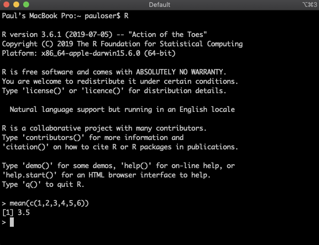
While most all of our efforts will be confined to using R through RStudio, the point of bringing up these other ways of working with R is to emphasize that R, by itself, is entirely text-based. Without an additional integrated development environment (IDE) like R Studio, it doesn't even recognize the mouse!
An entirely text-based application may seem like a throw-back to the days of old when MS-DOS ruled the world, and Apple and Windows operating systems were still finding their footings. Indeed, the great masses of computer users rarely run text-based programs anymore. Instead, they use programs that provide intuitive and easy-to-use graphical user interfaces (GUIs), full of windows, colorful icons, buttons, etc.
Text-based programs, on the other hand, generally have a steeper learning curve -- but they also offer tremendous flexibility, application, and speed. As such, even today, they are frequently the programs of choice for the power users and computer gurus of the world.
You can think of working with R as a conversation. When you start R (or R Studio), you are presented with a prompt -- an invitation to say something to R. Upon typing some command or expression, R produces some response. Then you get another prompt, and the process starts all over again.
While R is well more powerful than a scientific calculator, it can certainly function as one, when desired. Suppose you want R to perform a simple addition problem, like $1 + 1$. Simply type 1+1 at the prompt, and hit enter to see the answer:
> 1+1
[1] 2
For the moment, you can ignore the "[1]" that precedes the answer of "2". Some input expressions we will deal with later can cause R to produce many, many values in response. The "[1]" in this case simply means that the "2" seen to its immediate right is the first value output in response to "1+1".
Of course, we can do more than add. R supports all of the regular arithmetic operators (addition, subtraction, multiplication, and division).
> 1+1
[1] 2
> 2+3
[1] 5
> 2+3
[1] 5
> 2-3
[1] -1
> 2*3
[1] 6
> 2/3
[1] 0.6666667
> 2^3
[1] 8
R also supports some arithmetic operations you may not have known about.
> 17 %/% 5
[1] 3
> 17 %% 5
[1] 2
The %/% above performs the operation of integer division, which is identical to regular division, except it throws away any remainder.
The %%, on the other hand, outputs just the remainder of the related quotient.
We can combine multiple operations into a single mathematical expression, of course. When doing so, order of operations are preserved -- that is to say, things inside parentheses are evaluated first, multiplication and division happen before addition or subtraction, exponentiation happens before multiplication or division, and so on...
> 2 + 3*(1 + 5)^2
[1] 110
R is aware of some important mathematical constants. To use $\pi$ in an expression, for example, one just types "pi":
> 2*pi
[1] 6.283185
In addition to the simple operators and constants discussed above, R has many, many functions that one can use to build more complicates expressions. For example, one may wish to create an expression involving square roots, trigonometric functions, or logarithms. The following example calculates the value of $$\sin 3\pi/2 + \ln e^5 - \sqrt{4}$$
> sin(3*pi/2) + log(exp(5)) - sqrt(4)
[1] 2
More information on any of these functions can be found by typing the function name preceded by a "?" character. So for example, suppose we were interested in finding out how to change the base for the log function from the default $e$ to some other value. As such, we might type "?log" at a prompt, whereby we will be presented with an entire web page detailing everything we might want to know about the log function and all its variants and related functions. Try it!
The value of an expression can be assigned to a variable for later use. You can think of a variable as a box with a particular name. When we assign a value to a variable, we are essentially storing that value in the corresponding box.
In R, there are some limitations to the variable names one can use. Valid names consist of letters, numbers, and the dot (period) or underline characters. They must start with a letter or a dot not followed by a number. As examples, a name such as ".2way" would not be valid, while way_2 would be just fine.
There are also some reserved words that can not be used:
TRUE    NA             if        in
FALSE   NA_integer_    else      next
NULL    NA_real_       repeat    break
Inf     NA_complex_    while
NaN     NA_character_  function
To assign a value to a variable, one can use either the "=" or "<-" symbol, in a manner consistent with the following examples:
> x <- 3 + 4
> x
[1] 7
In this example, $7$ is stored as the value associated with variable $x$. Note that the assignment doesn't produce any visible output. To verify that $x$ has the value $7$, we type $x$ at a separate prompt.
Here's a slightly different example:
> y = 14 / 2
> z = y + 3
> z
[1] 10
Here, we use the alternate assignment operator ("="). We first assign the value of $7$ to $y$, and then $z$ is assigned the sum of $y$'s value and $3$. Neither of the assignments result in any visible output, so we type $z$ as a third input to verify things went as planned.
Notice that "=" in R does not mean "equals" in the mathematical sense. For this reason alone, many people prefer the "<-" form of the assignment operator.
Just as one can take something out of a box and replace it with something else -- one can re-assign a variable to a different value, as shown below.
> radius = 3
> 3.14 * radius^2
[1] 28.26
> radius = 5
> 3.14 * radius^2
[1] 78.5
Importantly, R is not limited to only associating a single value with a variable. It may associate a variable with a data set of many, many values. Let's make a simple data set (called a vector in R) consisting of the first five primes: 2, 3, 5, 7, and 11 and store it in a variable named $x$.
> x <- c(2,3,5,7,11)
> x
[1] 2 3 5 7 11
Here again, notice the first line only stores the values in the variable $x$, so to see the "value" of the vector $x$, we type just x on a separate later line.
We will talk more about vectors later, but let's take a look at a few basic ideas concerning them.
If we want to access to an individual element of a vector, we use square brackets. As an example, suppose one wishes to know the second element of the vector $x$ defined above. The following will do the trick:
> x[2]
[1] 3
We can find multiple elements of a vector in a similar way. Suppose one wishes to find the values of $x$ in the 3rd, 5th, and 4th positions (note: a more popular word for "position" in this context is index) in that order. The following code accomplishes this:
> x[c(3,5,4]
[1] 5 11  7
In the same way that the previously mentioned functions like sin(), log(), and sqrt() could be applied to individual values, other functions can be applied to entire data sets (e.g., vectors).
As an example -- in statistics, one is often interested in the average value of a data set, which is called its mean. In R, we can apply the mean() function to our data set $x$, and store the value calculated in another variable $m$:
> m <- mean(x)
> m
[1] 5.6
R comes "pre-loaded" with a bunch of data sets for demonstration purposes. You can see a list of these data sets by typing the following:
> data()
Let's take a peek at one of these data sets -- one called simply "rivers" -- that contains the lengths of major rivers in North America. If you want to see all 141 river lengths (in miles), simply type "rivers" at the prompt:
> rivers
  [1]  735  320  325  392  524  450 1459  135  465  600  330
 [12]  336  280  315  870  906  202  329  290 1000  600  505
 [23] 1450  840 1243  890  350  407  286  280  525  720  390
 [34]  250  327  230  265  850  210  630  260  230  360  730
 [45]  600  306  390  420  291  710  340  217  281  352  259
 [56]  250  470  680  570  350  300  560  900  625  332 2348
 [67] 1171 3710 2315 2533  780  280  410  460  260  255  431
 [78]  350  760  618  338  981 1306  500  696  605  250  411
 [89] 1054  735  233  435  490  310  460  383  375 1270  545
[100]  445 1885  380  300  380  377  425  276  210  800  420
[111]  350  360  538 1100 1205  314  237  610  360  540 1038
[122]  424  310  300  444  301  268  620  215  652  900  525
[133]  246  360  529  500  720  270  430  671 1770
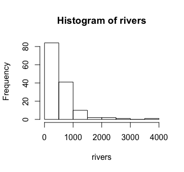
At the risk of getting ahead of ourselves, we can probably get a better feel for this data, however, by calculating both its mean and its standard deviation (another useful concept from statistics) and plotting a histogram (a nice way to visualize some data sets).
R makes doing these three things (and so many other things) exceedingly easy, as seen below.
Note, in the commands below, a # indicates a comment meant for humans and all text to the right of this symbol is ignored by R.
> mean(rivers)
[1] 591.1844
> sd(rivers)    # sd() is a function which finds standard deviations
[1] 493.8708
> hist(rivers)  # hist() is a function which plots histograms
I know what you are thinking -- what if you want to examine some data that's not automatically provided with R?
We'll answer this question more fully later -- but for now, if you just want to store a list of numerical values you found on the web somewhere into a vector so you can do all the things we just did to the rivers data set, don't worry -- there's a really easy way to do it!
We can use the scan() function, as shown in the example below:
Suppose you come across the following data set on the web, and wish to use it in R:
230, 146, 54, 463, 75, 377, 346, 77, 430, 30, 247, 251, 225, 488, 87, 424, 356, 80, 45, 171, 232, 466, 89, 209, 259
To store this data in a variable $x$, simply do the following:
Select all of the values and use "Ctrl-C" or "⌘-C" as appropriate, to copy the data from the webpage.
Then, noting that commas separate the values, type the following in R:
x = scan(sep=",")
Note: if there were no commas, you can just use x = scan().
A new prompt of "1:" will be shown.
> x = scan(sep=",")
1:
Use "Ctrl-V" or "⌘-V", as appropriate to then paste the data in R, and hit "Enter".
At this point R will display some number other than 1, followed by a colon.
> x = scan(sep=",")
1: 230, 146, 54, 463, 75, 377, 346, 77, 430, 30, 247, 251, 225, 488, 87, 424, 356,
80, 45, 171, 232, 466, 89, 209, 259
26:
The "26" above tells you that R has scanned 25 values and is waiting on you to type more if you wish, or to indicate that you are done by hitting "Enter" a second time. We have no more data, so hit "Enter" a second time.
That's it! Your data is now stored in the variable $x$.
We've just scratched the surface of R, but that will do for now.
If you are working in R-Studio, you can quit the program in the normal way (i.e., select "Quit RStudio" from the menu). Alternatively (especially if you are working with R in a console or other environment) -- you can simply type q() at the prompt.
In both situations, however, you will be asked if you wish to save your workspace image. If you answer in the affirmative, all of the variables with which you have been working will be automatically loaded, so you can pick up right where you left off...