
|
The relative frequency of an event (also called the empirical probability) is the number of times an event $E$ occurs divided by the number of trials conducted relative to a particular probability experiment. As an example, suppose we roll a die 5 times, yielding rolls 2, 6, 3, 6, 4. The relative frequency in this experiment of rolling an even value is thus $$P_e(E) = \frac{\textrm{# of rolls of 2's, 4's, and 6's observed}}{\textrm{total # of rolls}} = \frac{4}{5} = 0.80$$ where $P_e(E)$ here denotes the empirical probability of event $E$.
First, some observations are in order...
Note that as one runs more and more trials, the relative frequencies tied to an event will of course change. That said, over the long haul our intuition tells us that the overall relative frequency should settle down (in a limiting sense). This is often referred to as the Law of Large Numbers, which says that as the number of trials increases, $P_e(E)$ generally approach the true probability of event $E$. As an example, the more times a die is rolled, the closer we can expect the relative frequency of even rolls to get to $0.50$.
Importantly, know that the Law of Large Numbers does NOT say that if a particular event hasn't previously occurred as often as we might have expected, knowing the true probability associated with the event, that we are in any way "due" for this event to occur. Being "due" suggests the probability for the event to occur has somehow increased for these later trials, which should not be the case.
Additionally, as the fractions that calculate empirical probabilities only involve counts of things -- the probabilities should never be negative. Using an inequality to say the same thing more efficiently: If $C$ is any event, then $P_e(C) \ge 0$.
Third, recall that an event was defined as a subset of the sample space. Notably absent from this definition is any requirement that the event be a proper subset of the sample space (i.e., a set with a non-empty complement). Thus, one may consider the event $S$ that consists of the entirety of the sample space and thereby contains all possible outcomes. The occurrence of $S$ in any trial is clearly a certainty, and should have probability 100%. Writing this probability in decimal form (which will be a common practice going forward), we can again write this more efficiently as $P_e(S) = 1$.
Lastly, consider the relationship between the empirical probabilities observed for disjoint events $A$ and $B$ and the empirical probability of the event that corresponds to their union. An example might help us see this relationship more clearly: Suppose for a single roll of a die, event $A$ is associated with seeing an even value (i.e., 2, 4, or 6), while event $B$ is seeing the value 3. A die is rolled 100 times. In those 100 rolls, suppose $A$ occurs 47 times and $B$ occurs 19 times. As $A$ and $B$ are disjoint events, they can't both occur at the same time. Thus, either $A$ or $B$ occurs $47 + 19 = 66$ times. Consequently, $$P_e(A) = \frac{47}{100}, \quad \quad P_e(B) = \frac{19}{100}, \quad \quad \textrm{and} \quad \quad P_e(A \textrm{ or } B) = \frac{47+19}{100} = \frac{66}{100}$$
It should be clear from this example that, more generally, if $A$ and $B$ are disjoint events, then $$P_e(A \textrm{ or } B) = P_e(A) + P_e(B)$$
We are not limited to only considering two events $A$ and $B$, however. Suppose $\mathscr{C} = \{C_1,C_2,\ldots C_m\}$ is a collection of mutually exclusive events. This means that events in the collection are pairwise disjoint (i.e., $C_i \cap C_j = \varnothing$ for every possible pair $(C_i,C_j)$ of distinct sets in $\mathscr{C}$). Note that we can apply the above result repeatedly to find that $$P_e( C_1 \textrm{ or } C_2 \textrm{ or } \ldots \textrm{ or } C_m) = P_e(C_1)+P_e(C_2)+\cdots+P_e(C_m)$$
Remembering that when we consider the event $A \textrm{ or } B$, we are really considering their union (i.e., $P_e(A \textrm{ or } B) = P_e(A \cup B)$), we can both simplify and generalize the equations above by adopting the following notation:
Similar to how $\sum_{C \in \mathscr{C}} C$ describes the sum of all elements $C$ in a set $\mathscr{C}$, Let the union of all events $C$ in the collection $\mathscr{C}$ (even if the collection is infinite) be denoted by $\bigcup_{C \in \mathscr{C}} C$. Thus, if $\mathscr{C} = \{C_1, C_2, C_3, \ldots\}$, $$\bigcup_{C \in \mathscr{C}} C = C_1 \cup C_2 \cup C_3 \cup \cdots$$
Then, when considering any collection $\mathscr{C} = \{C_1, C_2, C_3, \ldots\}$ of mutually exclusive events (even an infinite collection), we expect the following to hold: $$P_e \left(\bigcup_{C \in \mathscr{C}} C \right) = \sum_{C \in \mathscr{C}} P_e(C)$$
Recall again that for a given random experiment and its sample space $S$, empirical probabilities over the long haul seem to get close to the "true" probabilities associated with the events in question. These "true" probabilities should, of course, share the same properties that are enjoyed by their corresponding empirical probabilities.
With this in mind, we are ready to make a definition that will make our meaning of the word probability more precise...
There are a host of useful properties that directly result from these three defining properties. The following details some of the more critical ones for our purposes:
A collection of events $\mathscr{C}$ is said to be exhaustive when the union of its events is the sample space itself. Thus, for any mutually exclusive and exhaustive collection $\mathscr{C} = \{C_1,C_2,C_3,\ldots\}$ relative to a given sample space, properties 2 and 3 in the definition of a probability set function require that $$\sum_{C \in \mathscr{C}} P(C) = 1$$ Notably, the set of all outcomes $x$ in a sample space $S$ is trivially a mutually exclusive and exhaustive collection of (simple) events, relative to $S$. Consequently, we may conclude that $$\sum_{x \in S} P(x) = 1$$
Equilikely Events If an event $E$ is the union of events $C_1 \cup C_2 \cup \cdots \cup C_r$ from an exhaustive and mutually exclusive collection $\mathscr{C} = \{C_1,C_2,\ldots,C_k\}$ relative to a sample space $S$, and all of events in $\mathscr{C}$ are equally likely, then $$P(E) = \frac{r}{k}$$ To see this, we first note that the previous result applies -- so we know $$\sum_{C \in \mathscr{C}} P(C) = 1$$ Additionally, if each such $C$ is equally likely, then we can find some constant $p$, so that $P(C) = p$ for all $C \in \mathscr{C}$.
Putting these two things together, we have $$\begin{array}{rcl} \displaystyle{\sum_{C \in \mathscr{C}} P(C)} &=& P(C_1) + P(C_2) + \cdots + P(C_k)\\ &=& \underbrace{p + p + \cdots + p}_{k \textrm{ times}}\\ &=& kp\end{array}$$ Thus $kp = 1$, which tells us that each $P(C)$ has the value $p = 1/k$. Applying property 3 again to $E$, we have $$P(E) = P(C_1) + P(C_2) + \cdots + P(C_r) = \underbrace{\frac{1}{k} + \frac{1}{k} + \cdots + \frac{1}{k}}_{r \textrm{ times}} = \frac{r}{k}$$For context, know that it is often the case with the random experiments that we will consider going forward that there is an equal likelihood of seeing any of the outcomes in the sample space. For example, in rolling a single die, each individual roll is assumed to be equally likely.
As the set of all outcomes are exhaustive and mutually exclusive, we can apply the above result to find the probability of any event $E$.
Consider the event $E$ of rolling an even number. The $r$ above is simply the count of outcomes that are even, while the $k$ above is the total number of outcomes in our sample space. As such,
$$P(E) = \frac{\textrm{count of outcomes in $E = \{2,4,6\}$}}{\textrm{total number of outcomes in $S = \{1,2,3,4,5,6\}$}} = \frac{3}{6} = 0.50$$$P(A) = 1 - P(\overline{A})$ for any event $A$ relative to a sample space $S$.
To see this, consider the collection $\mathscr{C} = \{A,\overline{A}\}$. This collection is certainly mutually exclusive as $A \cap \overline{A} = \varnothing$ and exhaustive as $A \cup \overline{A} = S$. Thus, by properties 2 and 3 of a probability set function, it must be the case that $P(A) + P(\overline{A}) = 1$. Subtracting $P(\overline{A})$ from both sides yields the desired result.
This result can often shorten the work needed to calculate probabilities. One should pay particular attention to this when finding probabilities of events described by using the words "at least", "at most", "more than", "less than", or "exactly". Consider the example that follows that involves rolling a single die. As a convenience, the probability of the simple event of rolling the value $x$ is abbreviated $P(x)$.†
Suppose one wishes to know the probability that the roll of a single die is "less than 6". Calling the described event $E$, we note that $E = \{1,2,3,4,5\}$, and thus $P(E)$ is the sum of probabilities of these mutually exclusive outcomes: $$P(E) = P(1)+P(2)+P(3)+P(4)+P(5) = \frac{1}{6} + \frac{1}{6} + \frac{1}{6} + \frac{1}{6} + \frac{1}{6} = \frac{5}{6}$$ However, consider how much briefer the calculation becomes when we realize the complement of $E$ is rolling a 6: $$P(E) = 1 - P(\overline{E}) = 1 - P(6) = 1 - \frac{1}{6} = \frac{5}{6}$$ Such savings in calculations don't always happen. For example, if the problem had been to find the probability of a roll "less than 2", using the complement would be more cumbersome than attacking the problem directly, as the complement of this event consists of four individual outcomes, while the event itself only involves two.
Still, in the cases where it helps -- it often helps immensely.
The probability of an event with no outcomes is zero.
This is a quick consequence of the last result. Denote an event associated with no outcomes in a given sample space $S$ by $\varnothing$. Then $\overline{\varnothing} = S$. By the result above, $P(\varnothing) = 1 - P(\overline{\varnothing}) = 1 - P(S) = 1 - 1 = 0$.
We say $A$ is a subset of $B$ when every element of $A$ is also an element of $B$, denoting this by $A \subset B$.
If event $A \subset B$, then $P(A) \le P(B)$.
As proof, note that $\mathscr{C} = \{A,\overline{A} \cap B\}$ is a mutually exclusive collection. Given that the union of the sets in $\mathscr{C}$ is $B$, property 3 of probability set functions tells us that $$P(B) = P(A) + P(\overline{A} \cap B)$$ Property 1 of probability set functions assures us that $$P(\overline{A} \cap B) \ge 0$$ Taken together, we have the desired result: $$P(B) \ge P(A)$$
$0 \le P(E) \le 1$ for every event $E$
This is another quick result. Noting that the $\varnothing \subset E \subset S$, we have by the last result: $P(\varnothing) \le P(E) \le P(S)$ Recalling that $P(\varnothing) = 0$ and $P(S) = 1$, we have the desired result.
The Addition Rule: $P(A \textrm{ or } B) = P(A) + P(B) - P(A \textrm{ and } B)$ for any events $A$ and $B$
This result requires slightly more work, but is well worth the trouble.
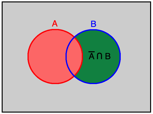
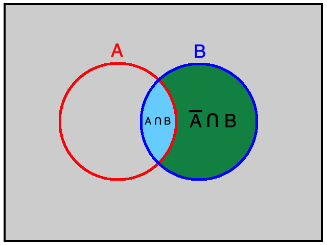
First, recall that $A$ or $B$ is the same event as $A \cup B$, and $A$ and $B$ is the same event as $A \cap B$. Thus, we seek to prove $P(A \cup B) = P(A) + P(B) - P(A \cap B)$ for any events $A$ and $B$.
Now consider the diagrams below.
Much of the study of statistics involves looking at certain situations and deciding whether or not under certain assumptions what is observed is unlikely. If the observations are "unlikely enough", one can feel fairly confident in rejecting the assumptions initially made. To setup a (somewhat arbitrary) standard for what we mean by "unlikely enough", let us call an event unusual if its probability is less than or equal to 0.05.