
|
Predict the output of each of the following when executed in R:
foo=function(d,n,max){
   nums=seq(from=1, by=d, length.out=n)
   return(nums[nums <= max])
}
foo(4,5,10)
what=function(n,a,b,c,d){
  x=(1:n)*5
  x=x[a:b]
  print(x)
  x=x[-c]
  print(x)
  x=x[x<d]
  return(x)
}
what(10,3,7,2,32)
fum=function(a,b) {
  a = a[a<b]
  return(a)
}
fum(3:7,(1:5)^2)
1 5 9
[1] 15 20 25 30 35
[1] 15 25 30 35
[1] 15 25 30
5 6 7
Suppose a jar contains $r$ red and $b$ blue marbles, and $n$ marbles are selected without replacement. Write an R function, marbles.probability(r,b,n,x), that returns the probability of getting exactly $x$ red marbles, similar to the function shown below:
> marbles.probability(8,9,5,2)
[1] 0.3800905
marbles.probability=function(r,b,n,x){
  p=choose(r,x)*choose(b,n-x)/choose(r+b,n)
  return(p)
}
Note, you can pass a vector to this function as well:
> marbles.probability(8,9,5,0:5)
[1] 0.020361991 0.162895928 0.380090498 0.325791855 0.101809955 0.009049774
Write an R function, choose.members(n,c,p), that returns the number of ways to choose members from an organization of $p$ people to serve on an executive committee consisting of $n$ "named positions" (e.g., president, vice-president, treasurer, and so on...), and $c$ at-large members of equal rank, as the sample output below suggests.
> choose.members(4,4,12)
[1] 831600
choose.members = function(n,c,p) {
  return(factorial(n)*choose(p,n)*choose(p-n,c))
}
Write an R function, number.sequence(n), that returns a vector that has the form $\{ 2^2 \cdot 3,\, 3^2 \cdot 5,\, 4^2 \cdot 7,\, 5^2 \cdot 9,\, \ldots \}$ and has exactly $n$ terms, as the sample output below suggests.
> number.sequence(5)
[1]  12  45 112 225 396
number.sequence = function(n) {
  squares = (2:(n+1))^2
  odds = 2*(1:n)+1
  return(squares * odds)
}
Write a function is.even(n) in R that returns TRUE when $n$ is even and FALSE otherwise. Then, using is.even(n), write a function evens.in(v) that returns a vector comprised of the even integers in a vector v of integers.
is.even = function(n) {
  return( n %% 2 == 0 )
}

evens.in = function(v) {
  return(v[is.even(v)])
}
The sequence of consecutive differences of a given sequence of numbers, $\{x_1, x_2, x_3, x_4, \ldots\}$, is the sequence $\{(x_2 - x_1), (x_3 - x_2), (x_4 - x_3), \ldots\}$.
Write a function consecutive.differences(v) that computes the consecutive differences of the elements of some vector $v$. An example application of this function is shown below:
> nums = c(1,6,7,9,11,15)
> consecutive.differences(nums)
[1] 5 1 2 2 4
consecutive.differences = function(v) {
  a = v[-1]
  b = v[-length(v)]
  return(a-b)
}
Assume that a data set is stored in the vector data in R. Write a function skewness(data) that calculates the skewness index ($I=\displaystyle{3(\bar x-Q_2)\over s}$) of the data set and returns either "The data is significantly skewed" or "The data is not significantly skewed" as appropriate.
skewness=function(data) {
  index=3*(mean(data)-median(data))/sd(data)
  return(ifelse(abs(index)>1,"The data is significantly skewed",
                             "The data is not significantly skewed"))
}
Describe what the following function does in the context of a statistics course. Be as specific as you can, without knowing the value of data
mystery=function(data){
  a=mean(data)-3*sd(data)
  b=mean(data)+3*sd(data)
  is.in=(data>a) & (data<b)
  print(sum(!is.in))
  return(data[is.in])
}
The function prints the number of outliers in data, and returns a vector identical to data, except with the outliers removed.
Write a function histogram.for.simulated.uniform.data(n,num.bars) that will simulate $n$ values following a uniform distribution and then plot the corresponding histogram. The histogram should have num.bars bars (although depending on the random data produced, it is possible that some interior bars might be zero-high). Additionally, the bars should appear "candy-striped", alternating between red and white colors, as the example below suggests:
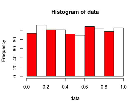
histogram.for.simulated.uniform.data = function(n,num.bars) {
  data = runif(n)
  bin.width = (max(data)-min(data))/num.bars
  cols = c("red","white")
  brks = seq(from=min(data),to=max(data),by=bin.width)
  hist(data,breaks=brks,col=cols)
}
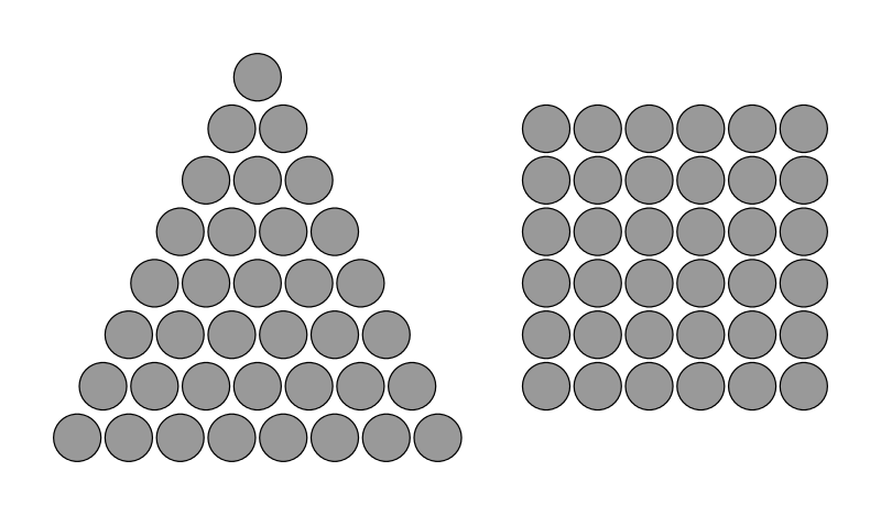
Triangles and Squares Revisited...
Recall a number of dots, $T_n$, of the form $\displaystyle{T_n = 1 + 2 + 3 + \cdots + n = \frac{n(n+1)}{2}}$ where $n$ is a positive integer, can be arranged in a triangular form with $n$ dots on each side.

Recall also, that some numbers of dots, like $36$, can form both a triangle and a square.
Suppose you wish to find all such numbers from 1 to $T_{1500000}$ using R. (Notably -- this is a range of values significantly longer than any row or column allowed in Excel!)
To this end, write the following three functions:
T(n), which returns $T_n$ for the given value of $n$.
is.perfect.square(x) which returns $TRUE$ if $x$ is a perfect square and $FALSE$ otherwise.
Hint: you may find it useful to use the R function trunc(x), which removes the decimal part of any real value, as squaring the truncated square root of $x$ will only equal $x$ if it is a perfect square.
nums.that.can.form.a.triangle.and.square(n), which will return all values of $T_k$ where $1 \le k \le n$ and $T_k$ is a perfect square.
What is the sum of the (only eight) $T_k$ values that are also perfect squares, where $k$ ranges from 1 to $1500000$?
is.perfect.square = function(x) {
  return(trunc(sqrt(x))^2 == x)
}

T = function(n) {
  return(n*(n+1)/2)
}

nums.that.can.form.a.triangle.and.square = function(n) {
  triangular.nums = T(1:n)
  return(triangular.nums[sapply(triangular.nums,is.perfect.square)])
}

sum(nums.that.can.form.a.triangle.and.square(1500000))
Chebyshev's Theorem puts limits on the proportion of a data set that can be beyond some number of standard deviations from its mean.
Recall, the mean and standard deviations associated with a sample of size $n$ are given by the following, respectively. $$\overline{x} = \frac{\sum x}{n} \quad \quad \textrm{and} \quad \quad s = \sqrt{\frac{\sum(x-\overline{x})^2}{n-1}}$$ where for each sum above, $x$ ranges over all data values in the sample.Also note that the built-in R functions mean(v) and sd(v) calculate these two sample statistics, $\overline{x}$ and $s$.
Use these two functions, to create a function proportion.within.k.std.dev.of.mean(sample.data,k), that finds the proportion of values in the vector sample.data that lie strictly between $(\overline{x} - k \cdot s)$ and $(\overline{x} + k \cdot s)$.
Store the following data in a vector named data, and then use this function to verify the proportion of the following data that falls within 1.1 standard deviations of the mean is 0.64.
16, 22, 31, 31, 35, 55, 72, 45, 11, 4, 70, 41, 71, 88, 21, 5, 86, 23, 91,
19, 63, 70, 17, 12, 49, 82, 40, 56, 25, 40, 37, 5, 83, 26, 16, 24, 3, 28,
10, 20, 61, 41, 10, 48, 61, 8, 69, 48, 26, 13, 82, 77, 11, 92, 88, 65, 40,
75, 88, 15, 34, 81, 15, 43, 69, 4, 58, 70, 50, 40, 77, 63, 42, 95, 52, 60,
79, 79, 73, 93, 18, 36, 83, 22, 53, 39, 10, 87, 78, 37, 34, 65, 100, 90,
100, 80, 28, 5, 59, 23
Note that the difference between the actual proportion found ($0.64$) and the bound established by Chebyshev's Theorem ($1 - 1/1.1^2 \doteq 0.1736$) is surprisingly large.
One might wonder how much lower one can make the actual proportion (and thus get closer to Chebyshev's bound), if you limit yourself to adding only a single value to the data set.
To this end, you run the following code:
proportion.with.extra.value = function(extra.val) {
  proportion.within.k.std.dev.of.mean(c(data,extra.val),1.1)
}

min(sapply(1:100,proportion.with.extra.value))
Rounded to the nearest thousandth, what minimum proportion results?
proportion.within.k.std.dev.of.mean = function(sample.data,k) {
  s = sd(sample.data)
  x.bar = mean(sample.data)
  return(sum((sample.data > x.bar - k*s) &
             (sample.data < x.bar + k*s))/length(sample.data))
}

data = ...

proportion.within.k.std.dev.of.mean(data,1.1)

proportion.with.extra.value = function(extra.val) {
  proportion.within.k.std.dev.of.mean(c(data,extra.val),1.1)
}

min(sapply(1:100,proportion.with.extra.value))
It can be difficult in R to view and make sense of a table with a very large number of rows and columns. Often, one is interested in identifying the cells of the table with the largest values. This is especially true when these represent frequency counts of certain combinations of categorical variable values.
Write a function dominant.cells(t,k) that reports, in decreasing order, the top $k$ cell values in a two-dimensional table $t$, along with their respective factor combinations, in a manner similar to that shown below:
> # First, let's create a new (random) table:
> categoryA = factor(sample(1:4,size=1000,replace=TRUE))
> categoryB = factor(sample(5:8,size=1000,replace=TRUE))
> t=table(catA=categoryA,catB=categoryB)
> t
    catB
catA  5  6  7  8
   1 55 67 61 54
   2 66 50 64 81
   3 48 65 71 64
   4 58 58 65 73

> # Now, we apply our dominant.cells() function:
> dc = dominant.cells(t,5)
> dc
   catA catB Freq
14    2    8   81
16    4    8   73
11    3    7   71
5     1    6   67
2     2    5   66
Towards this end, you may find the order(v) function useful, which creates a permutation of vector $v$ that would (through subsetting) put its elements in order. An example follows:
> v = sample(1:10)
> v
 [1]  4  3  8  2  9  1  7 10  6  5

> order(v)
 [1]  6  4  2  1 10  9  7  3  5  8

> v[order(v)]
 [1]  1  2  3  4  5  6  7  8  9  10
Import the data set dominant.txt, and convert it to a table with the table() function. Then use your function to find the cells of this table with the top 5 counts.
Based on the result, what is the sum of both the top 5 frequencies seen in the table and the row and column pairs to which they belong?
(Note: the corresponding sum for the top 5 frequencies in the $4 \times 4$ table generated and shown above is 404.)
url =
   "http://math.oxford.emory.edu/site/math117/probSetRFunctions/dominant.txt"

dominant.df = read.table(url,sep="")
t = table(dominant.df)

dominant.cells = function(tbl,k) {
  tbl.df = data.frame(tbl)
  freq.order = order(tbl.df$Freq,decreasing = TRUE)
  reordered.tbl = tbl.df[freq.order,]
  return(reordered.tbl[1:k,])
}

dominant.cells(t,7)

    categoryA categoryB Freq
473        23        46   47
296        26        40   42
683        23        53   42
579         9        50   41
836        26        58   41
299        29        40   40
597        27        50   40

# Ans:
Summing the numbers in only the first 5 rows under
categoryA, categoryB, and Freq, we get 567

In doing so, make the assumption that during the peak weeks of the shower, the times meteors will be visible to your telescope are uniformly distributed.
Note, as the time differences between successive sightings of meteors you have seen in the past are not distributed in a manner that you recognize (e.g., they are certainly not normally distributed), you decide to simulate a bunch of time differences by generating $n$ randomly chosen, but uniformly distributed times that on average are $k$ minutes apart, and then calculating the differences desired.
Armed with these simulated time differences, one can estimate the probability that one must wait $x$ minutes (or longer) to see a meteor. Write an R function p.value.estimate(x,k,n) that simulates the appropriate differences and returns this probability.
Rounded to two decimal places, what is the estimate produced by this function for the probability of waiting 45 minutes or longer between meteor sightings when the true difference between meteor sightings is 12 minutes, based on 100000 simulated differences?
Hint: There are multiple approaches you can take, but a particularly expeditious one makes use of the cut() and table() functions in R!
p.value.estimate = function(x,rate,n) {
  times = sort(rate*n*runif(n))
  times.between = times[-1] - times[-length(times)]
  counts = table(cut(times.between,breaks=c(0,x,max(times.between)),labels=FALSE))
  return(counts[2]/n)
}

p.value.estimate(45,12,100000)

1-pexp(45,1/12)  # <-- (for confirmation) this is the true p.value

# Ans: 0.02  (rounded to two decimal places)
Benford's Law can often be applied to data that spans several orders of magnitude -- things as diverse as populations of countries, loan amounts approved by a bank, river drainage rates, etc. Shockingly, it tells us that in these situations the leading digit of any particular element has a much larger chance of being a 1 than any other digit -- somewhere around 30% of the time! Indeed, Benford's law suggests that 1 will be the most common leading digit, followed by 2 (around 17.6% of the time), and 3 (12.5%), and so on -- with leading digits of 9 only happening around 4.8% of the time.
Check out this video to learn more:
You decide you want to test the claims made in the video above, so you write a function first.digit(n) that returns the leading digit of $n$, and then -- knowing that you need a data set that spans several orders of magnitude -- you apply it to all powers of $2$ from $2$ to $2^{500}$
As a hint for how to find the first digit of a number $n$, note that $\log_{10} n$ rounded down gives one less than the number of digits of $n$. (By the way, the R function trunc() will round down positive integers.).
Use your function to find the probability that a randomly chosen power of $2$ from $2$ to $2^{500}$ starts with a $1$. Then, find the probability that such a number will start with a $9$. What is the sum of these two probabilities (to the nearest hundredth)?
first.digit = function(x) {
  num.digits = trunc(log(x,base=10))+1
  return(trunc(x/(10^(num.digits-1))))
}

powers = 2^(1:500)
first.digits = sapply(powers,first.digit)

(sum(first.digits == 1)/500 + sum(first.digits == 9)/500)

★ At a magic show, a magician hands two sealed envelopes to a man and a woman in the audience, respectively. He then asks a child in the audience to pick some random value between 1 and 999, and shout it out to the audience. The child randomly chooses the number 547. (To make things more exciting, try the trick with your own chosen number.) After the audience hears the child's number, the magician instructs the man to open up his envelope and read aloud and follow the instructions inside. He does so, saying the following:
Write the digits of the chosen number so that they decrease from left to right.
Find the number whose digits are the reverse of the number formed in the previous step.
Given the two numbers just found, subtract the smaller one from the larger one.
Find the number whose digits are the reverse of the difference just found.
Add the last two numbers together (i.e., the difference and the "reversed" difference) and then shout this number to the audience.
Following the instructions, the man yells out "1089". The magician then directs the woman to open her envelope and reveal what is written inside. Of course, to the amazement of the crowd, the number "1089" is written on the sole piece of paper inside her envelope. (What happened with your chosen number?)
Wondering if every possible number the child could have chosen results in the same $1089$, you decide to replicate things in R...
Write the following functions:
digits.of(n), which returns a vector with the digits of the integer argument $n$ as its elements. Importantly, if $n=0$, the function should return a one-element vector equivalent to c(0). The following provides an example of its application:
digits.of(56789)
[1] 5 6 7 8 9

digits.of(0)
[1] 0
num.from.digits(digits), which does the reverse of digits.of(). Given a vector whose elements are single digits, this function returns the value they would form if placed side by side in the same order they appear in the vector. An example of this function's application is shown below
num.from.digits(c(5,6,7,8,9))
[1] 56789
trick(n), which applies the directions the man read to the crowd so that it can return the last number he calculated and shouted to the audience. In the story, the initial value picked by the audience member was 547. As such, it should be the case that
trick(547)
[1] 1089
Just in case you have any doubts, note that the final value is indeed $1089$ as predicted, as the following calculations show:
Number with digits decreasing: 754
754 - 457 = 297
297 + 792 = 1089
You apply the trick to all of the values from 1 to 999 with
results = sapply(1:999,trick)As you guessed, many of the answers are 1089 -- but surprisingly not all of them!
What is the second most common result when the trick is applied to these numbers?
Also -- and just for fun -- look at all of the values that didn't produce 1089 by running
which(results != 1089)Is there some easy-to-state restriction the magician could have insisted upon when asking the child to pick his initial number, so that this trick ALWAYS works?
digits.of = function(n) {
  num.digits = ifelse(n==0,0,trunc(log(n,base=10))+1)
  ks = num.digits:1
  digits = (n %% (10^ks)) %/% (10^(ks-1))
  return(digits)
}

num.from.digits = function(digits) {
  num.digits = length(digits)
  summands = digits*10^((num.digits-1):0)
  return(sum(summands))
}

trick = function(n) {
  step1Num = num.from.digits(sort(digits.of(n),decreasing = TRUE))
  step2Num = num.from.digits(reverse(digits.of(step1Num)))
  step3Num = step1Num - step2Num
  step4Num = num.from.digits(reverse(digits.of(step3Num)))
  step5Num = step3Num + step4Num
  return(step5Num)
}

results = sapply(1:999,trick)
summary(factor(results))

which(results != 1089)