
|
Predict the output of each when executed in R.
> nums = c(6, 7, 4, 9) %/% c(1, 2)
> nums[c(TRUE, FALSE, FALSE, TRUE)]
> nums = c(6, 7, 4, 9) %% c(2, 3)
> nums[! c(TRUE, FALSE, FALSE, TRUE)]
> nums = sqrt(c(5, 8, 11, 24) + c(4, 1))
> nums[c(TRUE, TRUE, FALSE, TRUE)]
> nums = c(3, 1, 5, 4) + 2
> nums[c(TRUE,FALSE,TRUE,FALSE)]
> set=paste(1:6,rep(c("A","B"),times=3))
> set[c(2,3,5)]
> x = c(1,4,5,2,3,7,0,9)
> sum(x > 5)
a) 6 4
b) 1 0
c) 3 3 5
d) 5 7
e) "2 B" "3 A" "5 A"
f) 2
Write R code to find the number of times $3$ occurs in a given vector $v$.
If the vector $v$ is as given below, the number of times $3$ occurs in $v$ is $21$.
v = c(5,4,1,1,1,5,1,5,3,2,4,1,4,3,2,1,5,1,3,4,
      1,1,4,1,3,5,4,3,5,3,3,3,2,2,5,3,3,4,3,2,
      2,1,5,3,5,2,3,5,3,5,4,3,1,2,2,3,3,4,2,5,
      2,1,1,1,1,4,5,1,5,5,5,5,4,4,5,4,2,2,2,1,
      5,5,1,2,5,3,4,5,4,5,3,1,3,4,1,3,2,1,2,4)
Suppose $v$ has been defined in R with
> v = c(2,5,3,6,8,9,1,10)What command in R will return the vector with every multiple of 3 greater than the average value of $v$ removed?
Answers vary, but both of the following work:
v[!((v %% 3 == 0) & (v > mean(v)))]
v[((v %% 3 != 0) | (v <= mean(v)))]
Write R code to find the second highest value in a given vector $v$.
If $v$ is defined as shown below, the second highest value it contains is $94$.
v = c(87,86,8,36,77,38,38,15,36,20,91,77,78,25,
      29,65,96,91,69,10,29,38,2,72,13,73,68,78,
      66,8,9,50,11,9,77,66,53,15,47,1,26,37,36,
      50,39,13,94,77,59,8)
Suppose the following definitions have been made in R:
variables = c("x","y","z")
subscripts = 1:4
Create a vector that consists of every combination of a variable $x$, $y$, or $z$ and subscript $1$, $2$, $3$, or $4$.
Here's one way (there are others):
variables = c("x","y","z")
subscripts = 1:4
paste0(rep(variables,each=length(subscripts)),"_",subscripts)
When executed, this displays the vector:
[1] "x_1" "x_2" "x_3" "x_4" "y_1" "y_2" "y_3" "y_4" "z_1" "z_2" "z_3" "z_4"
Create the following character vectors of length $30$:
("label 1","label 2", ..., "label 30")
Note that for each element above, there is a single space between label and the number following.
("fn1","fn2", ..., "fn30")
In this case, for each element above, there is no space between fn and the number following.
Use the paste() and paste0() functions.
What command in R will find the number of elements in the below vector that are greater than 70 and less than 90?
> v = c(90,75,99,65,76,82,85,70,86,94,93,81,
        89,58,61,96,62,77,94,52,89,78,99,76,
        56,91,78,78,99,72,92,77,74,64,77,91,
        93,67,54,53,65,57,83,89,65,54,84,70,
        83,94,90,82,82,55,81,99,89,90,59,86,
        78,99,55,86,74,58,87,71,84,91,75,54,
        82,66,89,91,93,76,73,67,68,83,96,54,
        86,80,58,85,82,86,85,94,95,
        87,60,74,87,54,88,67)
# Both of the following methods will work, although the first is more direct:

> sum(v>70 & v<90)         # method 1
[1] 48

> length(v[v>70 & v<90])   # method 2
[1] 48
Note, when finding mean(v) for the vector below, the result is NA given that there are NA and NaN values present in v. Use appropriate subsetting to find the mean of the values in v, ignoring any NA or NaN values that are present.
> v = c(1,5,5,1,4,1,9,1,6,1,7,NA,NaN,NA,4,2,1,3,7,8,
        6,5,8,8,2,2,5,5,7,9,5,9,10,1,NaN,9,9,5,1,NA,
        1,1,8,6,8,6,NA,NaN,4,5,7,2,NaN)
> mean(v)
[1] NA
> mean(v[!is.na(v)])
[1] 4.888889
Write R code to produce a vector of the elements (ordered from least to greatest) that are common to both a given vector $v$ and some other given vector $w$.
If $v$ and $w$ are defined as seen below, the desired vector of common elements will be equivalent to c(1,43,85).
v = c(8,92,1,50,36,29,1,64,50,15,1,8,22,85,
      1,15,22,57,43,22,64,8,1,78,85,1,99,15,
      36,92,50,36,1,57,92,29,64,99,36,22,57,
      15,78,99,99,64,15,57,22,8,78,36,78,15,
      50,50,92,57,85,50,22,57,78,92,71,78,50,
      85,22,36,92,15,57,78,78,64,29,15,92,99,
      29,57,29,50,71,99,22,99,92,50,36,64,50,
      99,71,1,92,57,1,29)

w = c(31,7,19,13,49,43,25,43,97,25,43,25,73,
      67,55,13,91,7,19,85,13,19,79,85,79,37,
      67,91,55,31,55,49,91,1,7,97,97,55,85,1,
      31,25,31,13,19,37,73,7,97,49,43,85,49,
      85,25,43,37,97,61,1,97,61,85,55,91,31,
      25,85,7,55,37,37,13,55,55,79,85,19,19,
      73,85,31,37,31,43,37,55,73,25,37,37,19,
      67,79,73,73,31,61,91,85)
Often in statistics, one needs to modify a given data set before using it to make some computation.
With this in mind,† and given this data set, use R to remove all of the following:What is the sum of the squares of the remaining elements?
As a test case for your code, if one does the same thing to this smaller data set, the sum of squares that results is 22463.
†Admittedly, the modifications asked for in this problem are a bit contrived -- but they serve as good practice in using vector functions, logical operators, and subsetting in R.
# after storing the data set values in a vector named data
# i.e., data = c(378, 428, 367, ...)
# do the following calculations:

d0 = sort(data)
d1 = d0[!duplicated(d0)]
d2 = d1[!((d1 > 3*min(d1)) & (d1 < 10*min(d1)) & (d1 %% 2 == 0))]
d3 = d2[!((d2 > 0.7*max(d2)) & (d2 < 0.9*max(d2)) & (d2 %% 2 == 1))]
ans = sum(d3^2)
ans
When data values are arranged from least to greatest, the middle value (presuming it exists) is called the median. This median will prove "central" to our study of statistics.
However, the values immediately around the median rarely, if ever, get examined. Seeking to correct that apparent injustice (if only for one problem), use R to find the sum of the middle 5 terms of this data set, when arranged from least to greatest.
# after storing the data set values in a vector named data
# i.e., data = c(67, 928, 111, ...)
# do the following calculations:

data = sort(data)
n = length(data)
mid.pos = (n %/% 2) + 1       # since n is odd
sum(data[mid.pos + (-2:2)])
The binomial distribution in statistics is closely connected with the coefficients seen in the $n^{th}$ powers of the binomial $(x+y)$. The first few powers of this binomial are shown below $$\begin{array}{rcc} (x+y)^0 &=& 1\\ (x+y)^1 &=& x+y\\ (x+y)^2 &=& x^2 + 2xy + y^2\\ (x+y)^3 &=& x^3 + 3x^2y + 3xy^2 + y^3\\ (x+y)^4 &=& x^4 + 4x^3y + 6x^2y^2 + 4xy^3 + y^4\\ (x+y)^5 &=& x^5 + 5x^4y + 10x^3y^2 + 10x^2y^3 + 5xy^4 + y^5\\ (x+y)^6 &=& x^6 + 6x^5y + 15x^4y^2 + 20x^3y^3 + 15x^2y^4 + 6xy^5 + y^6 \end{array}$$ Note that the coefficient on $x^{n-k}y^k$ in the expanded form of $(x+y)^n$ corresponds to how many ways we can select $k$ factors from the following $n$ factors to contribute a $y$ $$\underbrace{(x+y)(x+y) \cdots (x+y)}_{n \textrm{ factors}}$$ leaving the rest to contribute $x$'s.
Note that in the expanded form of $(x+y)^6$ shown above, the sum of the coefficients on terms involving exponents on $x$ that are multiples of $3$ is given by $1+20+1 = 22$.
With this in mind, use R to find the sum of the coefficients on the terms in the expanded form of $(x+y)^{37}$ that involve exponents on $x$ that are multiples of $3$?
(Curiously, the sum of all of the coefficients seen in the expanded form of $(x+y)^n$ is $2^n$. Can you see why?)
sum(choose(37,seq(from=0,to=36,by=3)))

# There are other ways of course, but this takes
# advantage of the symmetric nature of x and y
# in this problem
A 12-sided die has on each of its sides a different integer from 1 to 12, inclusive. Let $X$ be the random variable equal to the number of times the die must be rolled before it shows a prime value.
This is an example of a random variable that follows a geometric distribution. Note that on any particular roll, there is a probability $p = 5/12$ of rolling a prime value, and a probability $q = 7/12$ of rolling something else. Consequently, the probability the die must be rolled $k$ times before seeing a prime is given by $$P(k) = q^{k-1} \cdot p$$ Use R to find $P(5 \le X \le 80 \textrm{ and } X \textrm{ is even} )$ to 6 decimal places.
p = 5/12
q = 7/12
ks = seq(from=6,to=80,by=2)
sum(q^(ks-1)*p)
Later in our study of statistics, we will often find probabilities of certain events by finding areas under some given function over some interval on the $x$-axis. In some situations, calculus can help us find these areas quickly. However, even without calculus, one can approximate these areas to whatever level of precision might be desired.
One way to approximate the area under a positively-valued function over an interval on the $x$-axis is to first cut that interval into $n$ sub-intervals of equal length, and then consider the rectangles whose bases are these sub-intervals and whose heights are given by the value of the function at their right endpoints, as shown below. The sum of the rectangular areas will serve as the approximation to the area under the curve.
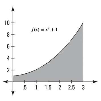
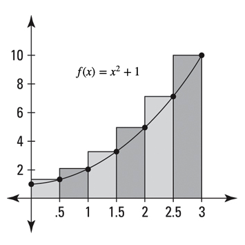
The images above show the area under the curve corresponding to the graph of $f(x) = x^2+1$ over the interval $[0,3]$ on the left, and the related rectangles when $n=6$ on the right.
Recalling the area of each rectangle is simply its base length times its height, we can see that the area is approximated by $$\mathscr{A} = (0.5)(0.5^2+1) + (0.5)(1^2+1) + (0.5)(1.5^2+1) + (0.5)(2^2+1) + (0.5)(2.5^2+1) + (0.5)(3^2+1)$$
Simplifying the above results in $\mathscr{A} = 14.375$. Compared to the exact area (found with calculus) of 12, we see our approximation is still a bit rough. However, we can do much better by choosing a larger value of $n$, which results in thinner rectangles and consequently, less "extra rectangular area" above the curve.
For large values of $n$, the calculation of the approximating area by hand is tedious -- but we can use R to evaluate the corresponding expression and make light work of this task. Use R to evaluate to the nearest thousandth the approximation for the aforementioned area (i.e, where $x$ ranges from $0$ to $3$) when $n=100$.
As a check on your work -- when $n=40$, R should produce an approximation of $12.340$ for this area.
n = 100
dx = 3/n
xs = seq(from=3/n,to=3,by=3/n)
ys = xs^2+1
sum(dx*ys)

The solution is relatively simple. Noting that a handshake is a mutual event that happens between two people, we simply need to know how many groups of two people can be chosen from a group of $2n$ people. As such, and letting $H(n)$ denote the number of handshakes that occur, we have $$H(n) = {}_{2n} C_2 = \frac{(2n)!}{2!(2n-2)!} = \frac{2n(2n-1)}{2}$$
The context of counting handshakes, however, opens the door to much more interesting problems. The following is one of the more well-known of these, called the "Hands Across the Table" problem (perhaps in reference to the 1935 movie of the same name?): Suppose there are $2n$ people seated around a circular table. In how many ways can all of them be simultaneously shaking hands with another person at the table in such a way that nobody's arms cross anyone else's?
The below diagram shows all of the cases for $n=1,2,3,\textrm{ and }4$:
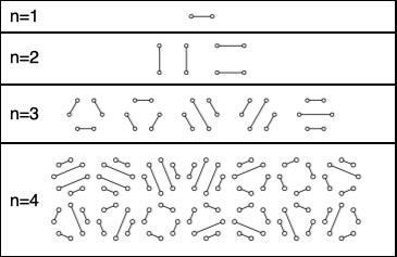
Denoting this number by $C(n)$, one might eventually discover the following (note, this is not a trivial conclusion -- but it is one that is fun to try to reproduce!) $$C(n) = \frac{{}_{2n} C_{n}}{n+1}$$
Upon finding the first few values of $C(n)$, (i.e., $1,2,5,14,42,\ldots$), one might notice that $C(n)$ grows much more quickly then $H(n)$. Use R to find the first value of $C(n)$ that is more than 1 million times the size of $H(n)$ for the same value of $n$.
n = 1:25
hs = 2*n*(2*n-1)/2
cs = choose(2*n,n)/(n+1)
all.bigger = cs[cs > 1000000*hs]
all.bigger[1]

Based on the work of Edgar Gilbert, Claude Shannon, and J. Reeds it was determined that 7 riffle shuffles are generally sufficient to thoroughly randomize a deck of cards. Of course, the shuffles involved in their work were not perfect riffle shuffles. We are curious how random a deck shuffled this many times appears if each shuffle is done perfectly.
To this end, use R to first construct a vector of strings in the following order:AH 2H 3H ... 10H JH QH KH AS 2S 3S ... 10S JS QS KS AD 2D 3D ... 10D JD QD KD AC 2C ...representing a deck with ace of hearts on top, followed by the 2 of hearts, 3 of hearts, and so on up to the king of hearts, followed by all of the spades, diamond, and clubs respectively, with each suit in a similar ascending order. (Hint: creative use of
paste0() and recycling can keep one from the tedium of typing this entire list into a vector.)
Then, use R to perform a perfect "out" riffle shuffle 7 times. Upon doing so, you should see that the top 5 cards are: $$AH \; 3H\; 5H\; 7H\; 9H$$ The rest of the cards exhibit a similar "lack of looking random".
One might wonder if there is something special about a deck with 52 cards that makes things look so "ordered" after 7 perfect riffle shuffles. With this in mind, let us modify the deck just used and then repeat the simulation.
Whereas a standard deck has ranks for each suit of Ace, 2, 3, ..., 10, Jack, Queen, and King, let us use a new (much larger) deck where the numerical ranks range from 2 to 100 (aces and face cards remain unchanged).
Correspondingly, modify the R code you used to create the vector of strings representing a standard deck so that it now produces the vector:
AH 2H 3H ... 100H JH QH KH AS 2S 3S ... 100S JS QS KS AD 2D ... 100D JD QD KD AC 2C ...representing the new, larger deck of $412$ cards. Again, the "Ace of Hearts" is the top-most card, while the "King of Clubs" is at the bottom of the deck.
Then, use R to perform 7 consecutive riffle shuffles on this new deck. What are the top 5 cards now?
ranks = c("A",2:100,"J","Q","K")
suits = c("H","S","D","C")
deck = paste0(ranks,rep(suits,each=103))
deck

n=length(deck)
out.shuffle.permutation = rep((1:(n/2)),each=2)+rep(c(0,n/2),n/2)

deck = deck[out.shuffle.permutation]   # Note, loops allow us to do this
deck = deck[out.shuffle.permutation]   # operation 7 times in a much more
deck = deck[out.shuffle.permutation]   # efficient way...
deck = deck[out.shuffle.permutation]
deck = deck[out.shuffle.permutation]
deck = deck[out.shuffle.permutation]
deck = deck[out.shuffle.permutation]
deck[1:5]
★ One hundred candidates apply for an open data analyst position at a company and will be interviewed in random order until the position is filled. Company policy dictates that the candidate be told at the end of his or her interview whether or not the company will be extending a job offer to that person. The interviewers decide on the following strategy in light of this policy:
The interviewers will interview the first $k$ of the $100$ candidates to get a feel for the quality of their candidate pool. All of these candidates, however, will not be offered the job. Then, they will continue to interview candidates until one of two things happen:
Note: you may assume that for any pair of candidates, one will always be better than another, allowing any set of interviewed candidates to be uniquely ranked.
Upon hearing the interviewers' strategy, management asks what value of $k$ will maximize the probability of offering the job to the best candidate in the entire pool.
With this in mind, let $p_k$ represent the probability of offering the job to the best candidate, when the first $k$ are interviewed but automatically rejected. Imagining the candidates waiting in a long line to be interviewed, the best candidate could be at any one of the $100$ positions in line with equal likelihood (i.e., each with probability $0.01$).

However, at different places in line, the probability of actually being selected can be different. For example, those in the first $k$ positions have no chance of being offered the job, while the probability of selecting a person past position $k$ is some positive value. Further, the probability of being offered the job diminshes as one gets closer to the end of the line, as it becomes more likely that someone earlier in the line has already been offered the job.
We are interested in the probability of the best candidate is offered the job. Given that the best candidate can only be at one of 100 disjoint positions -- we then seek the following sum: $$p_k = \sum_{i=1}^{100} P(\textrm{(the best candidate is at position $i$) } \boldsymbol{and} \textrm{ (offer made to candidate at position $i$)})$$ Recalling the multiplication rule (and abbreviating things slightly), this becomes $$p_k = \sum_{i=1}^{100} [P(\textrm{best candidate at $i$}) \cdot P(\textrm{offer made to $i$ } | \textrm{ best candidate at $i$})]$$ Again, each $P(\textrm{best candidate at $i$}) = 1/100$. However, the second factor on each term in the sum above is more interesting.
Recalling the first $k$ candidates interviewed are never offered the job, it must be true that $$P(\textrm{offer made to $i \le k$ } | \textrm{ best candidate at $i$}) = 0$$
For $i = k+1$, the probability the candidate at this position is offered the job when they are indeed the best candidate is a certainty, as such a candidate will clearly be better than any of the previous $k$ that have been interviewed. That is to say: $$P(\textrm{offer made to $i=k+1$ } | \textrm{ best candidate at $i$}) = 1$$
For $i > k+1$, the probability sought is different still, as one must account for the possibility of seeing a candidate anywhere from position $(k+1)$ to just before position $i$ that is better than all those candidates at earlier positions in the line, but still not the best candidate. (Hint: use a complement.)
Find an expression for the probability $p_k$ of offering the job to the best candidate in a pool of $100$ people. (Note of course, that the value of your expression will depend on the value of $k$.) Then, use R to determine the value of $k$ that maximizes this probability.
# The R work for this problem is actually minimal if you
# do some by-hand work playing with the probabilities first:

# Note, for a given k, the probability of finding the best is
# sum_{n=1}^N P(best at n AND select n)
# = sum_{n=1}^N P(best at n)*P(select n | best at n)

# P(select i | best at i) = 0 when 1 <= i <= k due to selection process

# P(select k+1 | best at k+1) = 1

# P(select k+2 | best at k+2) = 1 - 1/(k+1) = k/(k+1)
#   as only way you don't pick best is if 2nd best is at position k+1
#   chance of placing 2nd best in this one spot of k+1 spots is 1/(k+1)
#   then use complement

# P(select k+3 | best at k+3) = 1 - 2/(k+2) = k/(k+2)
#   as only way you don't pick best is if 2nd best is at position k+1 or k+2
#   (if 2nd best in first k, you make it to k+3)
#   chance of placing 2nd best in one of these two of k+2 spots is 2/k+2
#   then use complement

# P(select k+4 | best at k+4) = 1 - 3/(k+3) = k/(k+3)
#   as only way you don't pick best is if 2nd best is at position k+1, k+2, or k+3
#   (if 2nd best in first k, you make it to k+4)
#   chance of placing 2nd best in one of these 3 of k+3 spots is 3/k+3
#   then use complement
#
#   etc...
#
# adding these we have
#      (1/N)*1 + (1/N)*k/(k+1) + (1/N)*k/(k+2) + (1/N)*k/(k+3) + ... + (1/N)*k(N-1)

# so the probability we seek is = (k/N)*(1/k + 1/(k+1) + 1/(k+2) + ... + 1/(N-1))

# Note as k increases, the probability of getting the best
# should increase for a while (as you get a better feel for your "pool of candidates"),
# then decrease (as you increase your chances of having past the best one already)

N=100
# trying different k values reveals a max at k = 37, as seen below:
sum(35/(N*(35:(N-1))))
sum(36/(N*(36:(N-1))))
sum(37/(N*(37:(N-1))))
sum(38/(N*(38:(N-1))))
sum(39/(N*(39:(N-1))))
sum(40/(N*(40:(N-1))))  # loops can again make this process more efficient...