
|
What is the output if the following is executed in R?
loop.fun1 = function(n) {
   x = c(0,1,2)
   while (length(x) < n) {
        x = c(x,3)
    }
    return(x)
}

loop.fun1(6)
0 1 2 3 3 3
What is the output if the following is executed in R?
loop.fun2 = function(n) {
   x = 30
   while (x > 0) {
      x = x-n
   }
   return(x)
}

loop.fun2(7)
-5
What is the output if the following is executed in R?
loopy=function(n){
   x = 1:(2*n)
   while(x[1] < n){
       x = x[-1]
   }
  return(x)
 }

loopy(5)
5 6 7 8 9 10
Predict the output if the following is executed in R.
my.list=list(a=1:3,b=2:4,c=3:5)
x=c()
for (i in 1:length(my.list)){
   x=c(x,my.list[[i]])
}

x
[1] 1 2 3 2 3 4 3 4 5
Use a loop to write a function num.odd(v) that returns how many odd numbers there are in the vector v. Then, write a function num.odd2(v) that does the same thing without using a loop.
num.odd <- function(v) {
  count = 0
  for (x in v) {
    if (x %% 2 == 1) {
      count = count + 1
    }
  }
  return(count)
}
Now without a loop:
num.odd2 <- function(v) {
  return(sum(v %% 2 == 1))
}
The first two terms of the Fibonacci sequence are both ones. Subsequent terms of the sequence are found by summing the two terms immediately previous. Write a function fibonacci(n) that produces the first $n$ terms of the Fibonacci sequence for any $n \ge 3$.
fibonacci = function(n) {
   v = c(1,1)
   for (i in 1:(n-2)) {
      v = c(v,sum(v[c(length(v)-1,length(v))]))
   }
   return(v)
}
Write a function run.length(p) that simulates flipping a (possibly biased) coin with probability $p$ of landing heads until tails is seen, and returns the number of heads seen up to that point. Then, replicate the execution of this function 100 times with a fair coin and find the maximum run length seen.
run.length = function(p) {
  count = 1
  while (runif(1) < p) {
    count = count + 1
  }
  return(count)
}
max(replicate(100,run.length(0.5)))
A bag contains 3 red marbles and 1 white marble. A second bag contains 2 red marbles and 2 white marbles. Two marbles -- one from each bag -- are selected at random and swapped so that the marble from the first bag ends up in the second bag and the marble from the second bag ends up in the first. Then a marble is selected from the first bag and discarded. This swap-then-discard process is repeated a total of 4 times. Approximate the probability the 4th marble discarded is red by simulating this situation 1000 times.
bagFun = function() {
  bagA = c("R","R","R","W")
  bagB = c("R","R","W","W")
  removed = c()
  for (i in 1:4) {
    aPos = sample(1:length(bagA),size=1)
    bPos = sample(1:length(bagB),size=1)
    aItem = bagA[aPos]
    bItem = bagB[bPos]
    bagA = c(bagA[-aPos],bItem)
    bagB = c(bagB[-bPos],aItem)
    posToRemove = sample(1:length(bagA),size=1)
    removed = c(removed,bagA[posToRemove])
    bagA = bagA[-posToRemove]
  }
  return(removed[length(removed)] == "R")
}

sum(replicate(1000,bagFun()))/1000
Construct a function sample.space.for.n.sided.dice(n) that returns the a vector representing the sample space of all possible dice rolls of two $n$-sided dice (with faces labeled $1$ to $n$). As an example, the vector produced by sample.space.for.n.sided.dice(6) should contain one $2$, two $3$s, three $4$s, ..., two $11$s, and one $12$.
Hint: for each value that could be seen on the first die, you will have to consider each value that could be seen on the second die. Try accomplishing this by putting one for-loop inside the body of another for-loop.
sample.space.for.n.sided.dice = function(n) {
  sample.space = c()
  for (i in 1:n) {
    for (j in 1:n) {
      sample.space = c(sample.space,i+j)
    }
  }
  return(sample.space)
}

sort(sample.space.for.n.sided.dice(6))
Let us define a variant on a straight, called a "every-other-straight", where the 5 ranks present in the hand consist of "every other" rank, starting at the minimum rank seen in the hand. As an example, $(AH, 3S, 5D, 7D, 9C)$ and $(4D, 6D, 8H, 10C, QC)$ would both be every-other-straights.
In poker, straights may begin or end with an ace -- but to keep things simpler here, let us require that "every-other-straights" can begin with, but not end in an ace.
Use R to simulate one million 5-card poker hands. To the nearest thousandth, what is the proportion of "every-other-straights" seen?
deck = rep(1:13,times=4)  # note, suits aren't important

is.every.other.straight = function(hand) {
  for (i in 1:5) {
    if ( any(hand == i) &&
         any(hand == (i+2)) &&
         any(hand == (i+4)) &&
         any(hand == (i+6)) &&
         any(hand == (i+8))    )
      return(TRUE)
  }
  return(FALSE)
}

n = 1000000
sum(replicate(n,is.every.other.straight(sample(deck,size=5)))/n)
Remarkably, the Euclidean Algorithm allows one to find the greatest common divisor (GCD) of two numbers without ever factoring the numbers in question. This algorithm finds the GCD of two integers $a$ and $b$ by finding the remainder $r$ resulting from dividing $a$ by $b$, and then repeating this process letting $a = b$ and $b = r$, until the remainder is zero. The last non-zero remainder is the GCD. The calculations below demonstrate this process as they find the GCD of $90456$ and $2153106$:
90456 = 0 * 2153106 + 90456
2153106 = 23 * 90456 + 72618
90456 = 1 * 72618 + 17838
72618 = 4 * 17838 + 1266
17838 = 14 * 1266 + 114
1266 = 11 * 114 + 12
114 = 9 * 12 + 6
12 = 2 * 6 + 0

gcd(90456,2153106) = 6
You are interested in the average number of steps the Euclidean Algorithm takes when both numbers involved have 10 digits.
To this end, write the following two R functions:
num.steps(a,b), which calculates the number of steps the Euclidean Algorithm will need before the GCD is found. The example requires 8 steps (Note, each equation is considered a "step").
avg.steps(num.trials), which is the mean number of steps required for num.trials pairs of integers $a$ and $b$, randomly (and uniformly) chosen so that each has exactly 10 digits.
avg.steps()), with at least 1000 trials, and rounding to the nearest integer -- how many steps are required to find the GCD for pairs of numbers each 10 digits long?
(As a check of your work, if the two numbers only had 6 digits each, the average number of steps required is close to 12.)
num.steps = function(m,n) {
  cnt = 0
  while (n != 0) {
    m.next = n
    n.next = m %% n
    m = m.next
    n = n.next
    cnt = cnt + 1
  }
  return(cnt)
}

num.steps(90456,2153106)

avg.steps = function(num.trials) {
  sum = 0
  for (i in 1:num.trials) {
    m = sample(1000000000:9999999999,size=1)
    n = sample(1000000000:9999999999,size=1)
    sum = sum + num.steps(m,n)
  }
  return(sum/num.trials)
}

avg.steps(1000)
The Central Limit Theorem guarantees that the distribution of sample means from a normal population should itself be normal. Further, this distribution of sample means shares the same mean as the population, but has a smaller standard deviation. Indeed, if $\mu$ is the mean of the population and $\sigma$ is its standard deviation, then $\mu$ will also be the mean for the distribution of sample means, but its standard deviation will be given by $\sigma/\sqrt{n}$, where $n$ is the sample size.
Consequently, if one calculates the following statistic $$z = \frac{\overline{x} - \mu}{\displaystyle{\left(\frac{\sigma}{\sqrt{n}}\right)}}$$ for many, many different possible sample means $\overline{x}$ arising from equal-sized samples taken from the same population, the resulting distribution of these $z$-scores should "pile up" into a standard normal distribution.
While one might know (or have a good guess for) the mean value $\mu$ of a given population, having confidence in one's knowledge of the standard deviation can sometimes be harder to come by.
However, you know that the sample standard deviation provides an estimate of the population standard deviation. You are curious about the effect using the sample standard deviation in place of $\sigma$ in the above formula will have on the resulting distribution -- especially when the sample size is small (e.g., $n=5$).
To this end, create the following functions in R:
z(sample,mu,sigma), which calculates the $z$-score for the sample mean corresponding to the sample given by the vector sample. Note, mu and sigma provide the mean and standard deviation of the population from which the sample is drawn.
t(sample,mu), which performs a calculation almost identical to that of z(sample,mu,sigma), except that one has no knowledge of the standard deviation of the population, $\sigma$, and must therefore approximate this value with the sample standard deviation, $s$.
generate.zs(population,num.samples,sample.size), which constructs num.samples samples from the vector population, each of size sample.size. For each of these, a $z$-score given by the aforementioned z() function is calculated. All of the num.samples $z$-scores so calculated are returned in a single vector.
generate.ts(population,num.samples,sample.size), which essentially does everything the above described function zs() does, except that it uses the t() function instead of the z() function, and returns all of the num.samples $t$-values so produced in a single vector.
population to the vector including these values. Then, use the last two functions above (i.e., generate.zs() and generate.ts()) to create a collection of 10,000 $z$-scores and a collection of 10,000 $t$-values that both correspond to samples of size $5$, with the following:
zs = generate.zs(population,num.samples=10000,sample.size=5)
ts = generate.ts(population,num.samples=10000,sample.size=5)
You can see histograms showing the distributions of these two sets of values, if desired, with the following code:
brks = seq(from=min(c(zs,ts)),to=max(c(zs,ts)),length.out=70)
hist(ts,col=rgb(1,0,0,0.5),breaks=brks,main="",xlab="")
hist(zs,col=rgb(0,0,1,0.5),breaks=brks,add=TRUE)
legend("topright",
       legend=c("zs","ts","overlap"),
       col=c(rgb(0,0,1,0.5),rgb(1,0,0,0.5),"purple"),
       lwd=c(10,10,10))
box()
The resulting graphic should look somewhat similar to the following:
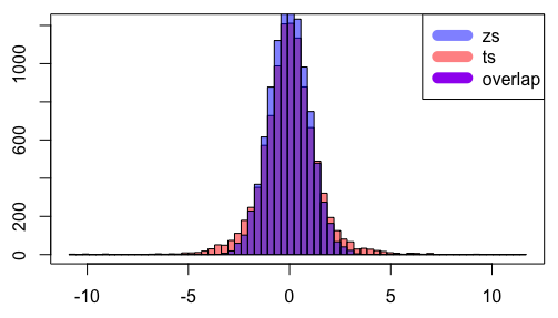
While the histograms will vary from one execution to the next due to the random sampling, one should generally see that the distribution of $t$-values is more spread out than that of the $z$-scores.
You wonder how much wider the $t$'s are, when compared to the $z$'s. To this end, recall that the standard deviation of the $z$-scores you generated should be very close to $1$. Rounded to the nearest tenth, what is the standard deviation of the collection of $t$-values you have generated?
z = function(sample,mu,sigma) {
  x.bar = mean(sample)
  return((x.bar - mu)/(sigma/sqrt(length(sample))))
}

t = function(sample,mu) {
  x.bar = mean(sample)
  s = sd(sample)
  return((x.bar - mu)/(s/sqrt(length(sample))))
}

z.test.statistics = function(population,num.samples,sample.size) {
  mu = mean(population)
  sigma = sd(population)
  collection = c()
  for (i in 1:num.samples) {
    collection = c(collection,z(sample(population,size=sample.size,
                                                  replace=FALSE),mu,sigma))
  }
  return(collection)
}

t.test.statistics = function(population,num.samples,sample.size) {
  mu = mean(population)
  collection = c()
  for (i in 1:num.samples) {
    collection = c(collection,t(sample(population,size=sample.size,
                                                  replace=FALSE),mu))
  }
  return(collection)
}

population = c( ... )  # <-- insert values from given link

zs = z.test.statistics(population,num.samples=10000,sample.size=5)
ts = t.test.statistics(population,num.samples=10000,sample.size=5)
sd(zs)
sd(ts)
You and a friend decide to play the following game, which involves flipping a fair coin until some sequence of heads and/or tails is seen. Both you and your friend pick a sequence of three heads and/or tails. You allow your friend to choose first. For example, maybe your friend picks $HHT$ and you pick $THH$. A coin is then flipped until either your sequence or your friend's sequence is seen. Whoever's sequence is first seen wins the game.
You employ the following strategy in picking your sequence. Recall your friend chose his sequence first -- suppose it is given by $\{x_1, x_2, x_3\}$ where each $x_i$ is either "heads" or "tails". You choose the sequence $\{y_1, y_2, y_3\}$ where $y_1$ is the opposite of $x_2$, $y_2$ is identical to $x_1$ and $y_3$ is identical to $x_2$.
There are only 8 possible sequences of heads and tails from which your friend can choose. Of these, you are curious as to when your strategy will (on average) result in a win for you.
To this end, write an R function coin.game(player1.seq) that takes a vector of 3 strings (each either "H" or "T") representing the sequence your friend chose, and returns either a $1$ or a $2$ depending on whether player 1 (your friend) or player 2 (you) won the game, respectively.
Then write an R function named proportion.player2.wins(n,player1.seq) that plays $n$ such games, and reports the proportion won by player 2 (i.e., you).
Finally, execute the following code to estimate (based on 100,000 trials) the proportion of the time you can expect to win the game in each of the aforementioned 8 cases:
proportion.player2.wins(100000,c("H","H","H"))
proportion.player2.wins(100000,c("H","H","T"))
proportion.player2.wins(100000,c("H","T","H"))
proportion.player2.wins(100000,c("H","T","T"))
proportion.player2.wins(100000,c("T","H","H"))
proportion.player2.wins(100000,c("T","H","T"))
proportion.player2.wins(100000,c("T","T","H"))
proportion.player2.wins(100000,c("T","T","T"))
Truncate each of these values to 2 decimal places. Then, ignoring any of these 8 values that suggest you will lose more often than win against your friend (i.e, throw out any proportions less than $0.5$), find the sum of the remaining proportions.
game = function(player1.seq) {
  flipped.middle = ifelse(player1.seq[2] == "H","T","H")
  player2.seq = c(flipped.middle,player1.seq[1],player1.seq[2])
  flips = sample(c("H","T"),size=3,replace=TRUE)
  game.won = FALSE
  while (TRUE) {
    if (all(flips == player1.seq)) return(1)
    if (all(flips == player2.seq)) return(2)
    flips = c(flips[2:3],sample(c("H","T"),size=1))
  }
}

proportion.player2.wins = function(n,player1.seq) {
  return(sum(replicate(n,game(player1.seq) == 2))/n)
}

ans.estimate = function() {
  props.wins = c(
    proportion.player2.wins(100000,c("H","H","H")),
    proportion.player2.wins(100000,c("H","H","T")),
    proportion.player2.wins(100000,c("H","T","H")),
    proportion.player2.wins(100000,c("H","T","T")),
    proportion.player2.wins(100000,c("T","H","H")),
    proportion.player2.wins(100000,c("T","H","T")),
    proportion.player2.wins(100000,c("T","T","H")),
    proportion.player2.wins(100000,c("T","T","T")))
  return(sum(props.wins))
}

ans.estimate()
Write an R function max.streak(p) that gives the length of the maximum "streak" of either all heads or all tails in 100 flips of a (possibly biased) coin whose probability of showing heads is $p$.
Use your function to determine the expected length (rounded to the nearest integer) of the maximum streak seen in 100 flips of a coin when the probability of seeing "heads" is $0.70$.
As a check of your work, note that the expected length of the maximum streak seen in 100 flips of a fair coin should be very close to 7.
max.streak = function(p) {
  flips = sample(c("H","T"),size=100,replace=TRUE,prob=c(p,1-p))
  max = 0
  pos = 1
  val = flips[1]
  cnt = 1
  while (pos <= 100) {
    if (flips[pos] == val) {
      cnt = cnt + 1
      if (cnt > max) {
        max = cnt
      }
    }
    else {
      val = flips[pos]
      cnt = 1
    }
    pos = pos + 1
  }
  return(max)
}

mean(replicate(10000,max.streak(0.7)))

A concordance is an alphabetical list of words present in a text, that shows where in the text these words occur.
Complete the body of the function concordance(url) shown below, so that it returns a list whose component names (i.e., tags) are the words encountered in the source text (specified by a url - for example, "http://math.oxford.emory.edu/myfile.txt"), and whose values are vectors whose elements are the positions of the words, as given by the numbers of words into the source text where the word in question is encountered.
As an example, if the source text started with "to be or not to be...", the concordance list would have "to" as one of its component tags, with the associated vector starting with positions 1, 5, ...
The tags in the list should be appear in order by their frequency in the source material, so that the beginning of the list shows the most frequently occurring words.
concordance = function(url) {
  txt = scan(url,"")
  # As a result of the above command, txt[i] now gives the ith word in the source text.

  # add your code here...

}
As an example, below shows the first 3 components of the list output by this function when applied to the text of the Gettysburg Address:
> concordance("gettysburg.txt")
Read 271 items
$that
 [1]  25  42  63  73  87  88  98 206 216 228 233 242 255

$the
 [1]  23 122 143 168 176 200 222 258 261 264 270

$we
 [1]  32  55  65  99 108 112 116 152 211 229
...
Once written, use this function to construct the corresponding concordance for Edgar Allen Poe's The Raven.
What is the sum of the elements in the vectors that correspond to the top 21 most frequent words in this poem?
Note: For the Gettysburg Address concordance, the sum of the elements in the vectors that correspond to the top 17 most frequent words would be 15337.
concordance = function(url) {
  txt = scan(url,"")
  word.list = list()
  for (i in 1:length(txt)) {
    word = txt[i]
    word.list[[word]] = c(word.list[[word]],i)
  }
  freqs = sapply(word.list,length)

  return(word.list[order(freqs,decreasing=TRUE)])
}

url = paste0(c("http://math.oxford.emory.edu/site/math117/",
               "labFactorsTablesListsAndDataFrames/raven.txt"))

c = concordance(url)

sum(sapply(c[1:21],sum))

# Ans: 186013