
|
Given the following data: 100, 95, 95, 90, 85, 75, 65, 60, 55. Find the median, mean, and mode. Is there a most appropriate measure?
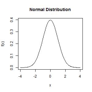
Make a sketch of the following, indicating the approximate locations for the mean, median and mode:
Given the data set: 1, 2, 3, 4, 5, 6, 7, 8, 9, 10, ''x''. Find the smallest positive integer value for ''x'' such that ''x'' is an outlier. Find the value for ''both'' definitions.
Given the following set of golf scores: 67, 70, 72, 74, 76, 76, 78, 80, 82, 85. Find the median, mean, mode, and standard deviation. What percentage of scores are in the interval of one standard deviation from the mean?
Give at least five uses and at least five misuses of statistics.
Give the four levels or categories of data and give an example of each.
Given the following grades on a test: 86, 92, 100, 93, 89, 95, 79, 98, 68, 62, 71, 75, 88, 86, 93, 81, 100, 86, 96, 52
A stem-and-leaf plot is a quick way to construct a histogram by hand, whereby one lumps together all values that have common leading digits up to some level of precision (i.e., the "stem") using the remaining digit(s) of each data value to form the "bars" (i.e., the "leaves"), as shown below for the data set $13,15,17,17,19,24,25,25,25,26,29,30,31,33,46,62$:
6 | 2
5 |
4 | 6
3 | 0 1 3
2 | 4 5 5 5 6 9
1 | 3 5 7 7 9
Make a stem-and-leaf plot that represents the test grade data.
10 | 0 0
 9 | 2 3 3 5 6 8
 8 | 1 6 6 6 8 9
 7 | 1 5 9
 6 | 8
 5 | 2
Find the mode, median, mean, range, standard deviation, and interquartile range
In R:

grades = c(86, 92, 100, 93, 89, 95, 79, 98, 68, 62, 71, 75, 88,
           86, 93, 81, 100, 86, 96, 52)

median(data)
mean(data)
range(data)
sd(data)
IQR(data)

# Sadly, the mode() function in R does something else.
# So you can write your own function, or if the data
# set is small enough (as it is here), you can use
# sort(data) to make it easier to count duplicate entries


TI-83:

Enter data in L1 with [STAT] : EDIT : Edit...
Then [STAT] : CALC : 1-Var Stats

This returns a scrollable list with:
 * median given by "Med"
 * mean given by x
 * range given by minX and maxX (technically, their difference)
 * standard deviation given by Sx (presuming the data is a sample)
 * interquartile range given by Q3 - Q1
Are there any outliers? Explain clearly.
What is an experimental design and why is it important? Describe a completely randomized experimental design and a rigorously controlled design.
Given this sample of freshman GPA scores:
2.2, 2.9, 3.5, 4.0, 3.9, 3.5, 2.9, 2.8, 3.1, 3.5, 3.8, 4.0,
3.8, 2.4, 3.9, 3.4, 2.8, 2.4, 1.8, 3.6, 3.1, 2.9, 3.8, 4.0
Is there an outlier? (Check both tests and explain)
Draw a frequency histogram using 5 to 6 categories. Be consistent with the rules for making histograms.
One set of boundaries includes: 1.65 to 2.05; 2.05 to 2.45; 2.45 to 2.85; 2.85 to 3.25; 3.25 to 3.65; 3.65 to 4.05, as shown below -- although a variety of answers will work.
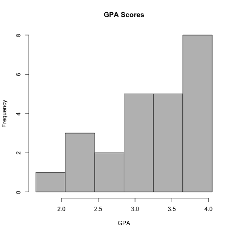
In R:
data = c(2.2, 2.9, 3.5, 4.0, 3.9, 3.5, 2.9, 2.8, 3.1, 3.5, 3.8, 4.0,
         3.8, 2.4, 3.9, 3.4, 2.8, 2.4, 1.8, 3.6, 3.1, 2.9, 3.8, 4.0)

hist(data,
     breaks=seq(from=1.65,to=4.05,by=0.40),
     col="gray",
     xlab="GPA",
     main="GPA Scores")
Is the distribution significantly skewed?