
|

Use R to test (at $\alpha = 0.05$) the claim that skittles candies are blended in equal proportions. What is the result?
The designer of the process by which skittles candies are made ensured the company that, with this process, they can expect the skittles candies produced to have a mean weight of 1.04 grams. The mean weight for the skittles in the sampled bag appears to be slightly higher. Does the sample provide significant evidence that the average weight of skittles is more than 1.04 grames? Use R to test an appropriate claim (at $\alpha = 0.01$).
What is the sum, rounded to 2 decimal places, of the $p$-value associated with the test conducted in part (a) and the test statistic and critical value for the test conducted in part (b)?
# import excel file skittles.xlsx using the "Files" panel...

counts = as.vector(table(skittles$colors))

# check assumptions (all E >= 5)
n = length(skittles$colors)
n*0.2 >= 5

test1 = chisq.test(counts,p=rep(0.2,times=5))  # GOF test

weights = as.vector(skittles$weights)

# check assumptions...
n >= 30

tt = t.test(weights,alternative="greater",mu=1.04,conf.level = 0.99)
test1$p.value + tt$statistic + qt(0.99,df=n-1)

# Ans: 50.25  (rounded to two decimal places)
R includes a dataset called iris that gives measurements in centimeters of the sepal length and width, and the petal length and width, respectively, for 50 flowers from three species (setosa, versicolor, and verginica) of iris plants.
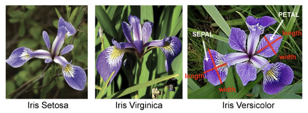
A friend claims it is easy to differentiate between the three species by their petal width, as iris virginica has a wide petal, iris setosa has a thin petal, and iris versicolor typically falls somewhere in between.
You decide to test the claim that the species and petal width are related (i.e., not independent) using the data found in the iris data set. However, the data needs to be altered slightly to suit your intended purpose:
Create a categorical variable for the plants in the dataset which identifies each as either "thin", "average", or "wide" in terms of their petal width, by determining whether the petal width is in the bottom third, middle third, or top third of all petal widths sampled. Then add this categorical variable to the data frame.
Finally, conduct an appropriate test to determine if there is any evidence that these categories of petal width are related to species type.
The $p$-value for this test appears exceedingly small, suggesting there is indeed a statistically significant relationship between petal width and species.
When the $p$-value is written in scientific notation, what is the exponent on $10$ used?
b1 = min(iris$Petal.Width)-1
b2 = quantile(iris$Petal.Width,1/3)
b3 = quantile(iris$Petal.Width,2/3)
b4 = max(iris$Petal.Width)+1

pet.cat = cut(iris$Petal.Width,breaks=c(b1,b2,b3,b4),
              labels=c("Thin","Average","Wide"))

iris$Petal.Cat = pet.cat
# check assumptions...
addmargins(table(iris$Petal.Cat,iris$Species))

summary(table(iris$Petal.Cat,iris$Species))  # independence test

# Ans: -56
Note, the file provided is incomplete -- not all subjects measured their body temperature at all of the times indicated. Any subject that is missing a body temperature on day 1 at 12am should not be considered when conducting the corresponding test. (Hint: one might find the is.na() function in R useful to this end.)
Make sure to check the assumptions for the test -- which, among other things, involves conducting a secondary hypothesis test -- before proceeding with the primary hypothesis test. Also, remember that checking for normality can be accomplished with a QQ-plot (see the notes on the qqnorm() function.
To the nearest thousandth, what is the sum of the two $p$-values that result? (i.e., one for the primary test and one for the secondary test.)
men = temps[temps$SEX=="M" & !is.na(temps$'DAY 1 - 12AM'),"DAY 1 - 12AM"][[1]]
women = temps[temps$SEX=="F" & !is.na(temps$'DAY 1 - 12AM'),"DAY 1 - 12AM"][[1]]
var.test(men,women)$p.value
# p-value = 0.7133
t.test(x=men,y=women,alternative="two.sided",conf.level=0.95,var.equal=TRUE)$p.value
# p-value = 0.1196

# Ans: 0.8329366 (sum of 2 p-values)
In computer science, a hash function is a function that turns its input into a number $h$ from $0$ to $(m-1)$, so that the input can be stored at position $h$ in some array of $m$ positions. For a hash function to work efficiently, the outputs for randomly chosen inputs should be as uniformly distributed between $0$ and $(m-1)$ as possible.
The following R function is equivalent to what the Java language uses as the default hash function when the input is a string of text.
hash = function(s,m) {
  a.vals = utf8ToInt(s)
  h = 0
  for (i in 1:length(a.vals)) {
    h = (31*h + a.vals[i]) %% m
  }
  return(h)
}
Test the claim that this function produces values that are uniformly distributed between $0$ and $9$ when $m=10$ by applying it to each word found here, and then conducting an appropriate hypothesis test.
To the nearest thousandth, what is the $p$-value for the test?
hash = function(s,m) {
  a.vals = utf8ToInt(s)
  h = 0
  for (i in 1:length(a.vals)) {
    h = (31*h + a.vals[i]) %% m
  }
  return(h)
}

url = "http://math.oxford.emory.edu/site/math117/labFactorsTablesListsAndDataFrames/words.txt"
words = read.table(url)
hash.vals = as.vector(table(factor(sapply(as.vector(words[[1]]),hash,m=10))))
chisq.test(hash.vals,p=rep(0.1,times=10))

# Ans: 0.267 (rounded to nearest thousandth)
In mathematics, there are often multiple paths to get to something of interest. Consider the vertex of a parabola. In algebra, one learns how to find where the vertex of a parabola is located by completing the square. However, in calculus there is a simpler way to get to the same end -- simply set the derivative of the corresponding quadratic function to zero and solve for $x$.
Finding the line of best fit for some given bivariate data is no exception. One way to find the equation $y = mx + b$ of this line, given data $\{(x_1,y_1), (x_2,y_2), (x_3,y_3), \ldots, (x_n,y_n)\}$, is to find $m$ and $b$ with the following formulas:
$$m = \frac{\sum (x_i-\overline{x})(y_i - \overline{y})}{\sum (x_i - \overline{x})^2} \quad \textrm{and} \quad b = \overline{y} - m\overline{x}$$That said, there is another way we could get at the same information -- one involving matrices. The explanation for why this next way works involves some concepts from both multivariable calculus as well as linear algebra, so we will not attempt an explanation here. However, the mechanics of the technique are easily understood, as the following will demonstrate.
Suppose one wishes to find the best fit line for the following data:
$$(1,0), (2,3), (3,7), (4,14), (5,22)$$To do so, we create a matrix $A$ whose first column consists of only $1$'s, and whose second column consists of the $x$-coordinates of the data. We also create a matrix $B$ consisting of a single column whose elements are the corresponding $y$-coordinates of the data.
$$A = \begin{bmatrix} 1 & 1\\ 1 & 2\\ 1 & 3\\ 1 & 4\\ 1 & 5 \end{bmatrix} \quad B = \begin{bmatrix} 0\\ 3\\ 7\\ 14\\ 22 \end{bmatrix}$$Using the standard notation $A^T$ for the transpose of a matrix (i.e., the matrix resulting from reversing the rows and columns of a given matrix), we compute the two matrix products $C = A^T \cdot A$ and $D = A^T \cdot B$:
$$C = A^T \cdot A = \begin{bmatrix} 1 & 1 & 1 & 1 & 1\\ 1 & 2 & 3 & 4 & 5 \end{bmatrix} \cdot \begin{bmatrix} 1 & 1\\ 1 & 2\\ 1 & 3\\ 1 & 4\\ 1 & 5 \end{bmatrix} = \begin{bmatrix} 5 & 15\\ 15 & 55 \end{bmatrix}$$ $$D = A^T \cdot B = \begin{bmatrix} 1 & 1 & 1 & 1 & 1\\ 1 & 2 & 3 & 4 & 5 \end{bmatrix} \cdot \begin{bmatrix} 0\\ 3\\ 7\\ 14\\ 22 \end{bmatrix} = \begin{bmatrix} 46\\ 193 \end{bmatrix} $$Finally, we find the product of the inverse of $C$ and $D$:
$$C^{-1} \cdot D = \begin{bmatrix} 5 & 15\\ 15 & 55 \end{bmatrix}^{-1} \cdot \begin{bmatrix} 46\\ 193 \end{bmatrix} = \begin{bmatrix} 1.1 & -0.3\\ -0.3 & 0.1 \end{bmatrix} \cdot \begin{bmatrix} 46\\ 193 \end{bmatrix} = \begin{bmatrix} -7.3\\ 5.5 \end{bmatrix}$$This last column matrix gives us the numbers we need to form the best-fit line:
$$\widehat{y} = 5.5x - 7.3$$Repeat this process for the bivariate data shown below. What is the predicted $y$ value to 2 decimal places using the best-fit line for $x=22$?
x	y
27.71	91.07
33.34	103.83
23.72	75.03
32.4	106.78
19.95	73.16
29.25	95.41
28.08	94.36
26.4	88.88
30.38	98.5
25.71	91.47
Answer to be posted soon!