
|
A normal distribution will be our first, and arguably most important example of a continuous probability distribution, so let's take a moment to describe what that is first...
A continuous probability distribution describes the probabilities of the possible values of a continuous random variable. Recall, that a continuous random variable is a random variable with a set of possible values that is infinite and uncountable. As a result, a continuous probability distribution cannot be expressed in tabular form. Instead, we must use an equation or formula (i.e., the probability distribution function -- in this context, also called a probability density function) to describe a continuous probability distribution.
Probabilities of continuous random variables (X) are defined as the area under the curve of its PDF. That is to say, $P(a \lt X \lt b)$ is the area under the curve between $x=a$ and $x=b$. Thus, only ranges of values can have a nonzero probability. The probability that a continuous random variable equals any particular value is always zero.
All probability density functions satisfy the following conditions:
For those familiar with calculus, we can also define a mean and variance for a continuous probability distribution with possible outcomes in the interval $[a,b]$, as the following (although, we won't use these definitions beyond their mention here). $$\mu = \int_a^b xf(x)dx \quad \textrm{ and } \quad \sigma^2 = \int_a^b (x - \mu)^2 f(x)dx$$ The standard deviation for a continuous probability function is still defined as the square root of the variance.
When creating a histogram associated with some continuous probability distribution the result is often "bell-shaped", similar to the shape seen in the histogram shown below. This is not surprising as the data in a sample, which in their own way are all individual estimates of some true population parameter (some good, some bad) often miss hitting their target exactly, and instead just fall somewhere nearby.
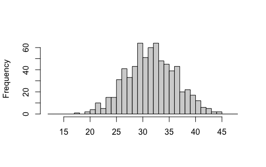
Of course, the values we see are unlikely to be too far away from the "true" average speed. Indead, the chances of seeing values farther and farther from the true value become less and less. We should consequently expect that the frequencies of data found farther and farther from the true value to fall accordingly.
One way for this to happen would be if the frequencies decreased in a manner proportional to the distance from the true value being estimated. However, with only this assumption the frequencies would eventually become negative, and that's impossible.
Under the assumption that all of the associated probabilities are positive, the best we can hope for is that the frequencies level off to a limiting value of zero, as the we get farther and farther from the true value.
We can make this happen if we require the rate at which the frequencies decrease be proportional instead to the product of the distance from the true value and the frequency itself. A random variable that follows a distribution where this is true is said to be normally distributed.
In the language of calculus, a probability density function $f$ which gives the frequencies of various values seen associated with a normally distributed random variable (called a normal distribution function) can thus be described by the following differential equation: $$\frac{df}{dx} = -k(x-\mu) f(x)$$
Solving this differential equation and writing the solution in a useful form is no simple task -- but the end result is that the function we seek can be expressed as: $$f(x) = \frac{e^{-\frac{1}{2} \left(\frac{x-\mu}{\sigma}\right)^2}}{\sigma\sqrt{2\pi}}$$ where $\mu$ is the expected value for the data (i.e., the "true" mean) and $\sigma$ is the associated standard deviation.
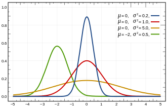
The below graphic shows a few normal distribution functions associated with various means and standard deviations.
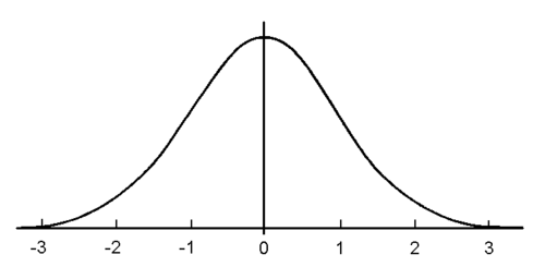
Importantly, all of the solutions for $f(x)$ found above are just tranformations of a simpler function, called the standard normal distribution function, whose equation is shown below. The graph of this function is called the standard normal curve. $$f(x)=\frac{e^{-\frac{1}{2}x^2}}{\sqrt{2\pi}}$$
Note that the transformations involved include only shifting left or right and stretching or compressing things vertically and horizontally, in a manner that keeps the area under the curve equal to $1$. In this way, the standard normal curve also describes a valid probability density function.
Using the definitions for mean and variance as it relates to continuous probability density functions, we can show that the associated mean for a standard normal distribution is 0, and has a standard deviation of 1.
The standard normal curve is shown below:
Note, it has the following properties...
Some additional properties of interest...
Because of the way in which every normal distribution curves is just some transformation of the standard normal curve, it must be true that for any normal distribution:
These approximations can, of course, be used in conjunction with the symmetry of a Normal distribution to approximate a few more proportions (such as the proportion of the distribution in the yellow, red, and blue vertical bands as shown below)
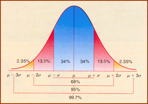
If upon looking at a distribution it appears to be unimodal, symmetric, and shaped in such a way that visually it appears to be "normally distributed", we can use the empirical rule to develop a test that can be applied to any data value in that distribution to determine whether or not it should be treated as an outlier.
Recall, according to the Empirical Rule, in any normal distribution we have the vast majority of our data (i.e., 99.7%) in the interval $(\overline{x} - 3\sigma,\overline{x} + 3\sigma)$. As such, approximating $\sigma$ by $s$ in a sample, we are suspicious of any data value outside of $$(\overline{x} - 3s,\overline{x} + 3s)$$ and consequently declare data values outside this interval to be outliers.
Incredibly important in statistics is the ability to compare how rare or unlikely two data values from two different distributions might be. For example, which is more unlikely, a 400 lb sumo wrestler or a 7.5 foot basketball player. It may seem like we are comparing apples and oranges here -- and in a sense, we are. However, when the distributions involved are both normal distributions, there is a way to make this comparison in a quantitative way.
Consider the following consequences of the Empirical Rule:
Data values more than 1 standard deviation away from the mean are relatively common, occurring with probability $0.32$. Values more than 2 standard deviations away from the mean are less common, occurring with probability of only $0.05$. Values more than 3 standard deviations away from the mean are very unlikely (so much so we mark their occurrence by labeling them as outliers), occurring with probability $0.003$.
Of course, we need not limit ourselves to distances measured as integer multiples of the standard deviation. With a bit of calculus, one can estimate the probability of seeing values more than $k$ standard deviations away from the mean for any positive real value $k$. In doing this, one finds (not surprisingly, given the shape of the distribution) that the probability continues to decrease as $k$ increases. As such, we can compare the rarity of two values -- even two values coming from two different distributions -- by comparing how many of their respective standard deviations they are from their respective means.
This measure, the number of standard deviations, $\sigma$, some $x$ is from the mean, $\mu$, in a normal distribution is called the $z$-score for $x$. The manner of its calculation is straight-forward,
$$z = \frac{x - \mu}{\sigma}$$
(Note, for folks that haven't had calculus, one can look up probabilities associated with a normal distribution using a normal probability table and $z$-scores. One can also use the normalcdf(a,b) distribution function on many TI calculators to find the probability of falling between $a$ and $b$ in a standard normal distribution.)
Some of the inferences we will draw about a population given sample data depend upon the underlying distribution being a normal distribution. There are multiple ways to check how "normal" a given data set is, but for now it will suffice to
Draw a histogram. If the histogram departs dramatically from a "bell-shaped curve", one should not assume the underlying distribution is normal.
Check for outliers. Carefully investigate any that are found. If they were the result of a legitimate error, it may be safe to throw out that value and proceed. If not, or if there is more than one outlier, the distribution might not be normal.
Check for skewness. If the histogram indicates a strong skew to the right or left, the underlying distribution is likely not normal.
Check to see if the percentages of data within 1, 2 and 3 standard deviations is similar to what is predicted by the Empirical Rule. If they aren't, your distribution may not be normal. Alternatively, if you have a larger data set, you should consider making a normal quantile plot. If your data is normally distributed, you can expect this plot to show a pattern of points that is reasonably close to a straight line. (Note: if your pattern shows some systematic pattern that is clearly not a straight-line pattern, you should not assume your distribution is normal.) Normal quantile plots are tedious to do by hand, but certain computer programs can produce them quickly and easily. (See the qqnorm() function in R.)