
|
Often, two variables will be related in that as one increases, the other generally increases -- or decreases. When this happens and points $(x,y)$ are plotted, where the $x$-coordinate is taken from the value of one of the variables, and the $y$-coordinate is taken from the corresponding value of the other variable, we sometimes see a (roughly) linear relationship. If the correlation between the two is significant, we can exploit it to make predictions about the value of one variable when we know the value of the other.
The aforementioned graph of points $(x,y)$ is referred to as a scatter plot. Some examples of scatterplots are shown below
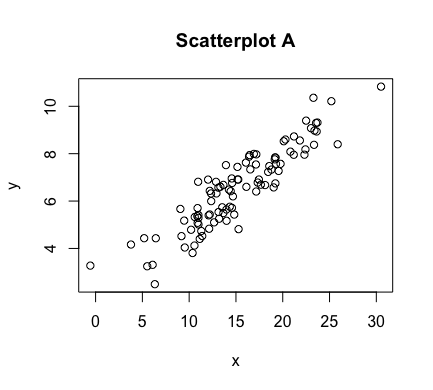
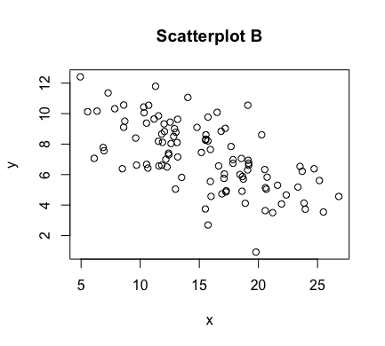
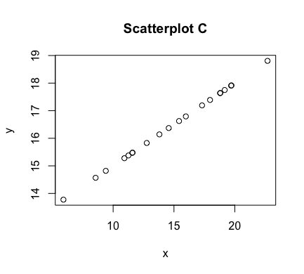
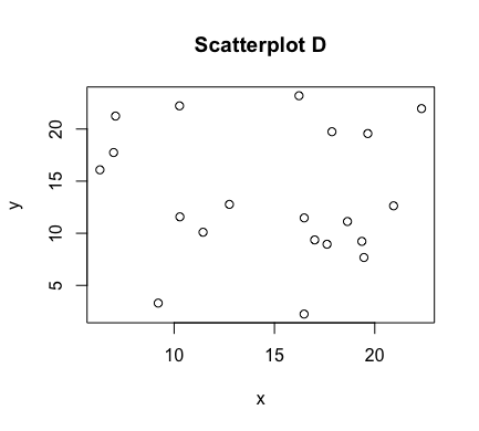
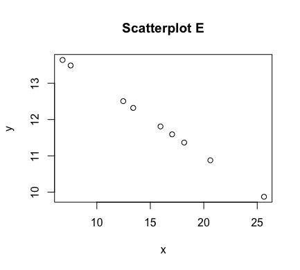
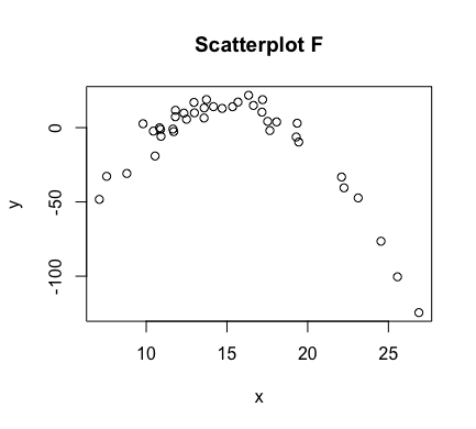
As can be seen above, the correlation between $x$ and $y$ is stronger in some of these scatterplots than others. In figures C and E, we have a perfect linear relationship. In these plots, the correlation is as strong as it can be. Scatterplots A and B have correlations that are less strong, with A perhaps being slightly stronger than B. In scatterplot D, there appears to be no correlation at all. In scatterplot F, there is correlation between $x$ and $y$, but it is not a linear one.
We can measure the strength and direction of a correlation with the Pearson product moment correlation coefficient. The population parameter that represents this is denoted by $\rho$, while the sample statistic for estimating $\rho$ is denoted by $r$ and calculated as follows:
$$r = \frac{\sum_{i=1}^n z_x z_y}{n-1}$$The maximum value of both $\rho$ and $r$ is $1$, which corresponds to a perfect positive correlation, where the points involved fall exactly on a line of positive slope (e.g., scatterplot C). Their minimum value of $-1$ corresponds to a perfect negative correlation, where again the points involved lie exactly on a line -- but this time, one of negative slope (e.g., scatterplot E). As $\rho$ and its estimating $r$ move towards $0$, the resulting scatterplots have an increased amount of "scatter" and the correlation becomes weaker and weaker, until there is no correlation at all (similar to scatterplot D).
The statistic $r$ can be calculated in a few different ways. For example it also equals $$r = \frac{s_{xy}}{s_x s_y}$$ where $s_x$ and $s_y$ are the sample standard deviations, as usual -- while $s_{xy}$ is the covariance given by $$s_{xy} = \frac{\sum_{i=1}^n (x_i-\overline{x})(y_i-\overline{y})}{n-1}$$ The covariance indicates how two variables are related. A positive covariance suggests the variables are positively related (when one goes up, the other does as well -- and if one goes down, the other matches that as well), while a negative covariance suggests the variables are inversely related (when one goes up, the other goes down - and vice-versa.).
Unfortunately, the value of the covariance depends upon the units used for $x$ and $y$. For example, if $x$ goes from being measured in feet to being measured in inches, the covariance for the same data will get multiplied by 12. Consequently, while it can provide an idea of whether one variable increases or decreases as the other variable changes, it is impossible to measure the degree to which the variables move together.
Dividing the covariance, $s_{xy}$, by the product $s_x s_y$, to form our correlation coefficient $r$ for the sample in question, corrects for this problem of being unit-dependent. (Algebraically, it introduces "unitless" $z$-scores into the expression). As such, $r$ is not affected by any changes of units used to measure either $x$ or $y$.
Additionally, given the symmetry of the formula that generates it, $r$ is also not dependent on which variable we refer to as $x$ and which we refer to as $y$.
One can conduct a hypothesis test to determine if there is significant evidence of a (non-zero) correlation between the variables associated with the $x$ and $y$ coordinates, provided one has met the following assumptions:
The null hypothesis for such a test is given by $H_0: \rho = 0$, with alternative $H_1: \rho \neq 0$. The test statistic follows a $t$ distribution with $(n-2)$ degrees of freedom, and is given by $$t = r\sqrt{\frac{n-2}{1-r^2}}$$
Importantly, correlation does not imply causation! That is to say -- just because $x$ is correlated with $y$ does not mean that $x$ causes $y$. :
The number of police active in a precinct is likely strongly and positively correlated with the crime rate in that precinct, but the police do not cause crime.
The amount of medicine people take likely also strongly and positively correlates with the probability they are sick, but the medicine does not cause the illness.
Data can sometimes also be spuriously correlated, but not actually have any relationship between them. As an example, between 2000 and 2009, the divorce rate in Maine and per capita consumption of margarine shows an amazingly strong negative correlation ($r = -0.992558$). What should we infer from this? Absolutely nothing.
One should remember that causal relationships can only be determined by a well-designed experiment.