
|
Suppose one wants to know the probability that the roll of two dice resulted in a 5 if it is known that neither die showed a 1 or a 6.
Note that knowing neither die showed a 1 or a 6 reduces the sample space normally associated with rolls of two dice down to:
$$\begin{array}{c|c|c|c|c|c|c} & 2 & 3 & 4 & 5 \\\hline 2 & (2,2) & (2,3) & (2,4) & (2,5) \\\hline 3 & (3,2) & (3,3) & (3,4) & (3,5) \\\hline 4 & (4,2) & (4,3) & (4,4) & (4,5) \\\hline 5 & (5,2) & (5,3) & (5,4) & (5,5) \\\hline \end{array}$$After shrinking the sample space, the rest of the calculation is routine. There are now only 2 cases out of 16 where the sum of the dice is 5. Thus, the probability we seek is $2/16 = 1/8$.
Now, more generally, consider the task of calculating the probability of some event $B$ under the condition that some other event $A$ has occurred.
We denote this probability by $P(B|A)$, calling the function applied a conditional probability function.
When considering $P(B|A)$ we know $A$ has occurred, which means our sample space essentially shrinks from what it previously was to just those outcomes present in $A$ itself.
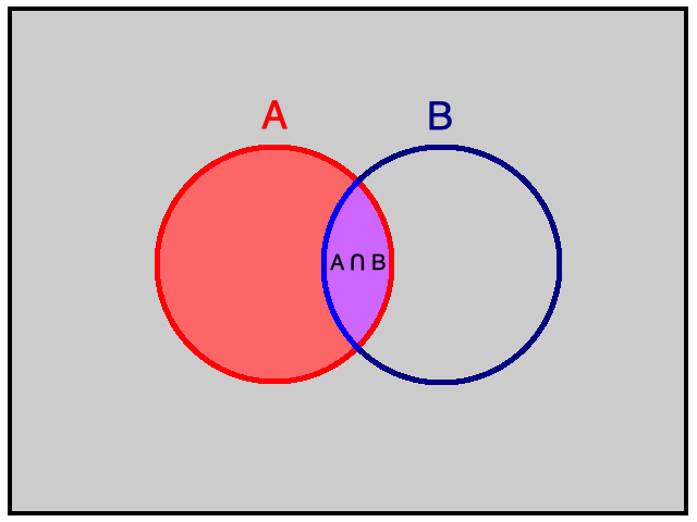
Revisiting the example above using this new notation, let $B$ be the event of rolling a sum of 5 on two dice; and let $A$ be the event where neither die rolled shows a 1 or 6. By examining the shrunken sample space, we previously found $$P(B|A) = \frac{2}{16}$$ However, there is another way to make this calculation when $P(A) \neq 0$. Consider the following: $$\frac{P(A \cap B)}{P(A)} = \frac{\displaystyle{\left(\frac{2}{36}\right)}}{\displaystyle{\left(\frac{16}{36}\right)}} = \frac{2}{16}$$
Similarly, we expect for any events $A$ and $B$ when $P(A) \neq 0$: $$P(B | A) = \frac{P(A \cap B)}{P(A)}$$ Multiplying the left and right sides above by $P(A)$ we have the following when $P(A) \neq 0$,† $$\displaystyle{P(A \cap B) = P(A) \cdot P(B|A)}$$
The above establishes the important rule shown below, which is especially useful for finding probabilities of compound events:
Of course, this rule is entirely symmetric as $A \cap B$ is the same as $B \cap A$. Thus, we also can say $P(A \textrm{ and }B) = P(B) \cdot P(A|B)$.
† : For completeness, note that if $P(A)=0$, we can still compute $P(A \cap B)$ -- just by different means. Recall that we have previously shown if $C \subset D$ then $P(C) \le P(D)$. Note that $C = A \cap B$ is a subset of $D = A$. Thus $P(A \cap B) \le P(A) = 0$. Since no probability is negative, it must then be the case that $P(A \cap B) = 0$.
We normally think of events $A$ and $B$ as independent when knowledge of one of these events occurring does not affect the probability that the other occurs.
It may not be clear what this means if either $A$ or $B$ is a null event -- as one would never have knowledge of a null event's occurance (remember null events never occur). For the moment then, presume these two probabilities are non-zero.
Under this presumption, when $A$ and $B$ are independent, we can write both $P(B|A) = P(B)$ and $P(A|B) = P(A)$, as both $P(B|A)$ and $P(A|B)$ are well-defined when both $P(A)$ and $P(B)$ are non-zero.
Consequently,
$$P(A\text{ and }B) = P(A) \cdot P(B|A) \quad \Longleftrightarrow \quad P(A\text{ and }B) = P(A) \cdot P(B)$$Let us now turn this into the definition for independence. That is to say,
Doing this is certainly consistent with our earlier notion of independence, but it also expands this idea now to null events. Specifically, it requires null events be independent of other events. Hopefully, one finds reasonable that the knowledge of one event's occurrence can't affect the probability of some other event that had zero probability of occurring in the first place.
To see how this definition requires null events be independent of other events, suppose $A$ is a null event and $B$ is any other event tied to the same sample space. Certainly then, we have $P(A) = 0$. Thus, the right side of the defining equation above (i.e., $P(A) \cdot P(B)$) equals zero.
It remains to show the left side must be zero as well. Again, recall that we have previously shown if $C \subset D$, then $P(C) \le P(D)$. Noting that $C = A \cap B$ is a subset of $D = A$, which has probability zero -- it must be the case that $P(A \cap B) \le 0$. As no probability is negative, we have $P(A \textrm{ and } B) = P(A \cap B) = 0$. As such, the left and right sides of the equation defining independence above agree, and $A$ is thus independent of $B$!
Turning our attention to a practical consequence of independence, consider the context of selecting members from a given population to decide if some characteristic is present in the members selected. Importantly, one can make this selection either with or without replacement. To see what this means, consider the following example:
Suppose one intends to test some selection from a group of batteries in order to classify them as either "good" or "defective". Suppose also that this group consists of 10 batteries, and 4 of them are defective. Note that the probability of drawing one of the 4 defective batteries from the group of 10 is 4/10 = 0.40. Suppose two batteries are selected.
One way in which this might happen is for the first one to be selected and tested and then returned to the group. Then a second battery is selected and tested in the same way. In this way, the probability of drawing a defective battery is identical for both selections. As the probability of drawing a defective battery on the second draw does not change from the probability of drawing a defective battery on the first draw, we note that the event of drawing a defective battery on the first draw and the event of drawing a defective battery on the second draw are hence independent.
However, one might not want to allow for the possibility that the same battery is tested twice. (If the context were different, and we were selecting people to complete a survey, instead of batteries, eyebrows would certainly be raised if we allowed a person t fill out the survey twice!) To accommodate this new restriction, one could set the first battery tested aside and then draw the second battery from the remaining nine. However, note that this changes the probabilities involved. If the first battery drawn was defective, the conditional probability that the second battery will be found to be defective is now $3/9 = 1/3$. If the first battery drawn was not defective, the conditional probability the second battery will be found to be defective is instead $4/9$, which is still different from the probability of $4/10$, that the first battery was defective. Consequently, the events of drawing a defective battery on the first and second draws, respectively, are not independent.
Different techniques must then be used in these two different circumstances. The former often leads to simpler calculations, but the latter is often more appropriate. Fortunately, the numerical difference between the two probabilities involved is very small when the population is large enough when compared to the sample size (i.e., the number of elements drawn from the population).
As a guideline, if the sample size is no more than 5% of the population size, the selections may be treated as independent, if desired, and the results are likely to still be close enough to the truth to be useful.