
|
An initial study of calculus can be miraculously distilled down to just a couple of carefully stated general problems.
The first such problem is this:
Given a point on the graph of some given function, what is the slope of the tangent line to the function at that point?
As simply stated as this problem is, its applications are huge and far-reaching. Let's consider just a couple of these applications:
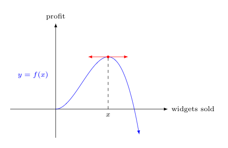
Optimization. Suppose the function in question gave the expected profit earned upon selling $x$ widgets at some company. One naturally would be interested in knowing how many widgets must one sell to maximize profit.
Notice how the slope of the tangent line at the highest point on the curve below is horizontal. Often, finding places where the tangent line has horizontal slope reveals maximum (and minimimum) values.
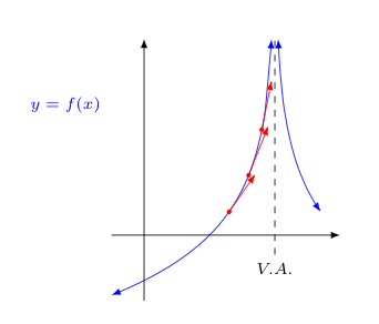
Graphing Functions. Knowing the slopes of tangent lines at various points on the graph of a function can help one better understand the graph of the overall function. For example, if we know that as we approach some $x$-value from the left, the slopes of the corresponding tangent lines increase without bound, then we can conclude there is a vertical asymptote at that $x$-value.
I know what you are thinking -- couldn't we just graph the function on our calculator to discover the same thing? Interestingly, the answer to that question is "No"!
Calculators can quickly calculate things, but sometimes they lie. There's of course no nefarious intent on their part -- but calculators often try to answer our questions using techniques that are not quite up to the task.
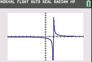
Want to graph a function? A calculator will basically plot a hundred points and connect the dots. If there is a vertical asymptote present and one of those hundred points doesn't happen to land exactly where the asymptote was, the calculator will miss it and draw the graph incorrectly.
An example is shown below, where one attempts to plot $y = 1/(x-2)$ on a calculator. Note how the curve on the calculator screen appears to makes a sharp turn around $(2,8)$, but this of course doesn't actually happen.
Understanding the nature of slopes of tangent lines to functions (and other things we can glean from calculus) can raise red flags when appropriate to alert us to not be so quick to believe what we see on our calculator screens.
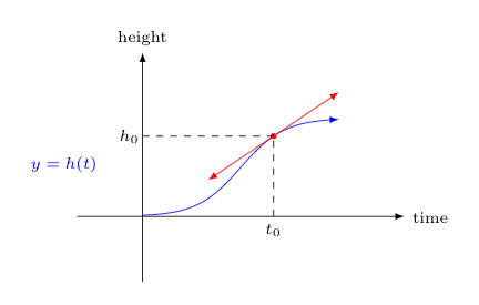
Instantaneous Velocity. Suppose that the $x$-axis now represents time, and the $y$-axis represents the position/height of some object -- perhaps a rising red balloon. The slope of the tangent line is then a distance traveled divided by an elapsed time and can thus be interpreted as a velocity.
Indeed, as we will soon see, the slope of the tangent line at $(t_0,h_0)$ corresponds to the instantaneous velocity this object is traveling at some time $t_0$.
In this particular case, the slope of the tangent line corresponds to the velocity with which the balloon is rising at the time $t_0$, when it is $h_0$ high.
Other Instantaneous Rates of Change. Of course, there is nothing special about thinking of the $x$ and $y$ coordinates as representing time and position/height, respectively.
Any two variables can be related in a similar way. In each case, the slope of the tangent line corresponds to the rate of change in one variable seen for a particular value of the other.
The table below suggests some possibilities:
| $y$ | $x$ | interpretation of tangent slope |
|---|---|---|
| amount of a drug in the human body | time | the rate of change in the amount of the drug at a particular time (i.e., drug absorption) |
| volume of water in a lake | depth | the rate of change in volume at a particular depth |
| charge passing through a section of wire | time | the rate of change in charge passing through the wire at a particular time (i.e., current) |
| pressure exerted on a material | volume of the material | the rate of change in pressure at a particular volume |
| mass of a rod (of non-constant density) | a position along the length of the rod | the rate of change of mass at a particular position along the rod's length (i.e., linear density at this location) |
Whenever we introduce a mathematical idea, we will always want to be as precise as possible in what we mean. Failing to do this can lead to the disaster of inconsistent conclusions -- a mathematical "sin", if there ever was one.
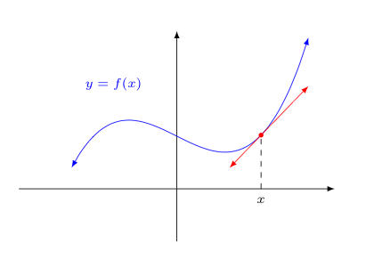
In the discussion above, we refer repeatedly to a tangent line to a function at some point. What do we actually mean by this? In geometry, one normally defines a tangent as a line that intersects a curve (typically a circular arc) at only one point. Will this definition suffice for our purposes? Consider the graph below.
.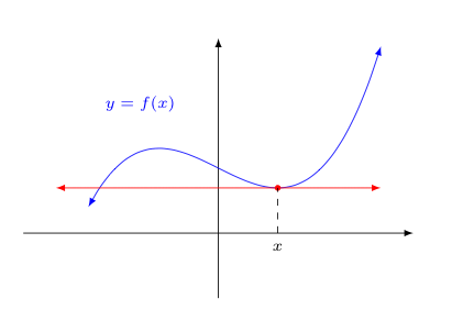
At the red point directly above $x$, the red line seems to be capturing the instantaneous rate of change in the height of the function (in that one instant, the function doesn't seem to be rising or falling). So in this sense, calling it a tangent line seems reasonable. However, the red line also intersects the curve in two places, which suggests the reverse if we adhere to the old geometric definition of a tangent line.
The solution, of course, is to define what we mean by a tangent line in a different way. We abandon the definition found in geometry textbooks for one more suited to the functions and applications found in calculus:
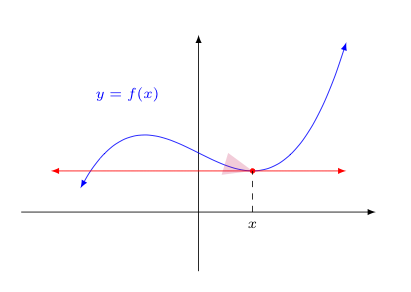
Definition: Let $\mathcal{C}$ be a curve and $\ell$ be a line that intersects $\mathcal{C}$ at some point $P$. Suppose that for every angle whose vertex is at $P$ and contains the line $\ell$, the curve $\mathcal{C}$ enters the angle. When this happens, we say that $\ell$ is the tangent line to $\mathcal{C}$ at $P$.
One should think carefully about what this definition says.
To help with your understanding, note how the angle shaded pink below was drawn to contain the red line. Now notice that the blue curve of $f(x)$ also enters this pink angle. Regardless of how thin this pink angle is made -- as long as it contains the red line -- the blue curve will always enter the angle. This makes the red line a tangent line for the purposes of discussions in calculus.
So how does one find the slope of a tangent line to a given function through a given point?
The slope of a tangent line is no different from the slope of any other line. For any two points $(x_1,y_1)$ and $(x_2,y_2)$ on a line, the slope is the constant ratio $m$, given by
$$m = \frac{y_2 - y_1}{x_2 - x_1}$$The problem is that we are typically only aware of one point through which the tangent line passes.
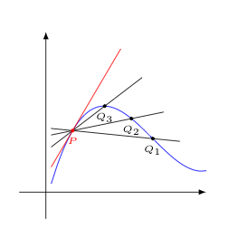
The standard approach is then to consider first a secant line that passes through the desired point on the graph of the function and one additional point not far from this point, as shown below.
The below image shows three such secants $\overline{P Q_1}$, $\overline{P Q_2}$, and $\overline{P Q_3}$. Note, the slopes of these secants do a better job of approximating the slope of the tangent line to the curve at $P$ shown in red as the second point $Q_i$ gets closer to $P$.
Let's take a closer look at one of these secant lines, and how one might find its slope. Consider the image below with point $P$ at $x=a$, and point $Q$ at distance $\Delta x$ to its right along the $x$-axis.
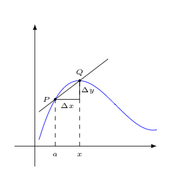
Note that if the blue curve is the graph of a function $f$, then the height of point $P$ is $f(a)$ and the height of $Q$ is $f(x)$ for some $x$ value.
This means that the "rise" in the function, $\Delta y$, as one goes from $P$ to $Q$ is given by $$f(x)-f(a)$$ As the "run" from $P$ to $Q$ is the difference of their $x$-coordinates, $x-a$, we have the slope (i.e., "rise over run") of the secant line given by $$m = \frac{f(x)-f(a)}{x-a}$$
We earlier said that the as the point $Q$ gets closer to $P$, the slope of the secant line does a better job of approximating the slope of the tangent line at $P$ (currently not drawn).
One might assume that the actual tangent slope would correspond to when $Q$ is at its closest to $P$ -- indeed, when $Q$ and $P$ are the same point.
However, this wrecks our expression above for the slope. At this moment, when $Q$ and $P$ are indistinguishable, $f(x) = f(a)$ and $x = a$, making both the numerator and denominator below zero.
$$m = \frac{f(x)-f(a)}{x-a}$$As such, the expression above for the slope is indeterminant when $x=a$.
Still, it appeared the secant slope was approaching something right before this sudden failure of evaluation...
If we could only find the value our slope expression was approaching as the horizontal distance between $P$ and $Q$ was getting closer to zero...
What we are seeing is the need to introduce the notion of a limit of an expression. In a nutshell, we want the limit of an expression at some value to give us the value of that expression that we would have expected to see, had it not been for the difficulties of indeterminant form or other problems.
While the calculation of almost every tangent slope to a curve will involve the evaluation of a limit under the surface somewhere -- the study of limits is not itself limited to this context.
As a quick example, consider the following expression, as $x$ gets closer and closer to $0$.
$$\frac{\sin x}{x}$$For any non-zero $x$, the expression above is well-defined. However, the moment $x=0$ we again get an indeterminant expression of "$0/0$".
Still, as one considers values of $x$ very close to $0$, the value of the expression appears to be very close to $1$, as the following table suggests:
$$\begin{array}{c|c} x & \sin(x)/x\\\hline 0.2 & 0.99335\\ 0.1 & 0.99833\\ 0.01 & 0.99998\\ 0.001 & 0.99999 \\ \end{array}$$While not proof, the above table certainly creates an expectation that at $x=0$, the value of the expression should have been 1, were it not for that pesky business of having a zero in the numerator and denominator.
In the next section, we will examine under what circumstances these expectations can be formed and when they can't. This will give us an intuitive understanding of what we intend when talk about limits.
Of course, the next step after gaining an intuitive understanding of what we mean by a limit will be to define things more precisely...