
|
As one motivation for the upcoming material, suppose we are interested in finding the area bound between the $x$-axis and some non-negative function on the interval $[a,b]$.
We might approximate this area by slicing it into vertical strips, approximating each of these strips with a rectangle of a similar height, and adding all of these rectangular areas together.
We can identify which strips we wish to use by partitioning the interval $[a,b]$ into $n$ sub-intervals.
To accomplish our partition, we select $x$-values, $x_1 \lt x_2 \lt x_3 \lt \ldots \lt x_{n-1}$, all of which are inside $[a,b]$. Then, we add to this set $x_0 = a$ and $x_n = b$.
The $n$ sub-intervals are then $[x_0,x_1], [x_1,x_2], [x_2,x_3], \ldots, [x_{n-1},x_n]$, with the $i$th sub-interval given by $[x_{i-1},x_i]$.
One can see the rectangular approximations to the vertical strips corresponding to one partition in the graphic below. Note, that in the picture all of the rectangles are the same width (this is called a regular partition), but we do not require that to be the case.
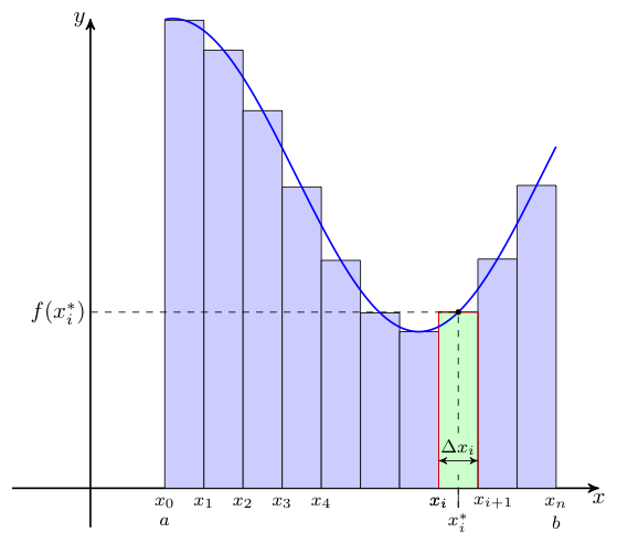
To find the height of the approximating rectangle for any such sub-interval, we note that we would certainly not want to use any value less than the minimum value obtained by the function on this sub-interval -- nor would we want to use any value greater than the maximum on this sub-interval. That said, any height attained by the function in the sub-interval will do nicely.
With this in mind, pick some $x^*_i$ in the $i$th sub-interval, $[x_{i-1},x_i]$, for each $i$ in $1,2,\ldots,n$, and let $f(x^*_i)$ be the height of the approximating rectangle.
In the above image, we pick the midpoint of the $i$th sub-interval to serve as $x^*_i$, but we could make other choices as well.
If we are to add up the areas of these rectangles to approximate the area under the curve, we will need to know their widths as well. Let us denote the width the the $i$th rectangle by $\Delta x_i$, as shown above.
Not surprisingly, of course, $\Delta x_i = x_i - x_{i-1}$.
For regular partitions, note that all $\Delta x_i$ correspond to the same width -- so in these instances, we may simply denote this width by $\Delta x$, dropping the subscript.
For non-regular partitions, there will be a largest value of $\Delta x_i$ seen. We call this value the norm of the partition, denoting this by $||\Delta||$.
Recall, we intend to add the areas of all of the rectangles to approximate the area under the curve. With that in mind, consider the area contributed by the $i$th rectangle. Of course, this area is simply the product of the rectangle's height $f(x^*_i)$ and its width $\Delta x_i$.
Summing over all $i = 1, 2, \ldots, n$, we have the following as the approximate area under the curve from $x=a$ to $x=b$:
$$\textrm{Approximate Area} = \sum_{i=1}^n f(x^*_i) \Delta x_i$$Of course, not all approximations are equal. Some are better than others. Think about the effects of the various choices we make in the formation of the sum above on how good the resulting approximation will be.
It should be relatively obvious that thinner rectangles leave less room for error when approximating the strip areas, and thus lead to a better overall approximation when added together.
For regular partitions, we can ensure that all of our rectangles become thin by simply having a lot of them.That is to say, presuming our partition creates $n$ sub-intervals, larger values of $n$ will generally lead to better approximations.
For non-regular partitions on the other hand, we can force all of the rectangles to become thin by requiring the norm to become small.
We also have some choice with regard to how we select $x^*_i$ for each sub-interval. The image shown at the top of this page showed each $x^*_i$ chosen to be the midpoint of its corresponding interval. This generally does a good job -- but one does have other options...
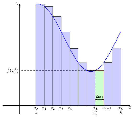
One could pick the left endpoint of each sub-interval (i.e., $x^*_i = x_{i-1}$) to determine the heights of the approximating rectangles. Alternatively, one could pick the right endpoint of each sub-interval (i.e., $x^*_i = x_i$) just as easily. These choices are shown below for the curve originally considered.
 |
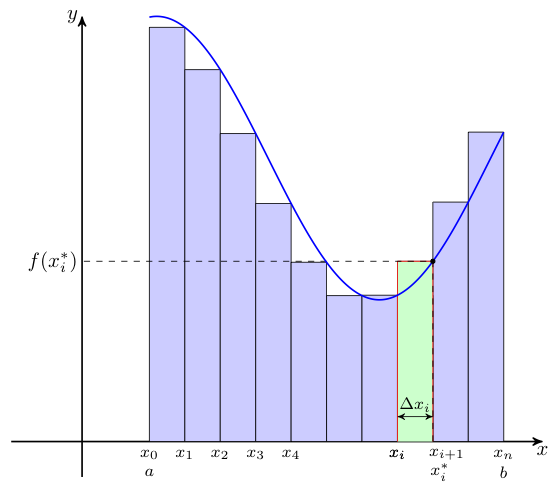 |
Note how when the function is decreasing, using the left endpoints creates an over-estimate of the area, while when the function is increasing, using the left endpoints creates an under-estimate of the area.
On the other hand, when the function is decreasing, using right endpoints creates an under-estimate, while when the function is increasing, they create an over-estimate.
Still, these three possible choices for $x^*_i$ (i.e., midpoint, left endpoint, or right endpoint of the corresponding sub-interval) are not the only ones one might consider.
Who knows -- maybe you'd prefer to pick as your $x^*_i$ that special value of $c$ guaranteed to exist by the mean value theorem relative to some antiderivative of the function in question and the $i$th sub-interval. I know what you are thinking -- that's a very strange (but oddly specific) suggestion for our choice of $x^*_i$. Oh what amazing things are yet to come!