

 |  |
Let us return for a moment to the notion of a permutation. Recall that applying a permutation to a set of $n$ elements would move each of these $n$ elements from their initial position to some final position, as suggested by the image below.
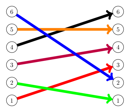
In this way, we can think of permutations in terms of a set of "input/output" pairs, where each possible initial position can be thought of as an "input" and the corresponding final position after the permutation has been applied, thought of as the "output".
Notice, in this case the set of all inputs here is $\{1,2,3,4,5,6\}$, as is the set of outputs.
Finding the value of $x^{-2}$ is another idea that can be thought of in terms of inputs and outputs. Here however, while we might take as inputs any real value $x \ne 0$, the outputs resulting from these inputs would only be positive real values.
Finding square roots, negating values, or finding their absolute values can all similarly be thought of in terms of finding some output for each of a given set of inputs.
Indeed, this idea of finding the output of some action on some input is pervasive in mathematics, so developing some common verbiage and notation for this general idea will be useful.
Towards that end -- while both the examples above and more that follow will involve finding numerical outputs from inputs that are also numerical -- we must be careful not to be too limited in whatever definitions we adopt. As we have seen, mathematics is not always just about numbers!
A means for producing some (single) output from some input is called a function in mathematics. We often use letters $f$, $g$, and $h$ to denote generic functions, although any letter will do. When the function's output has a clear interpretation, like volume or acceleration -- we often pick an abbreviating letter like $v$ or $a$, respectively.
To denote the output of some function $f$ corresponding to some input $x$, we write $f(x)$, reading this as "$f$ of $x$".
As examples, if $v$ is the function that gives the volume of a cube with input width $w$, we can say all of the following: $$v(2) = 8; \quad v(3) = 27; \quad v(w) = w^3$$
As additional verbiage, when we find the value of the output of a function $f$ for some input $x$, we also say we have "evaluated $f$ at $x$". In this way, the function $v$ above, when evaluated at $2$ is $8$. Similarly, $v$ at $3$ evaluates to $27$. Even more briefly, we might say "$v$ is $8$ at $2$" and "$v$ is $27$ at $3$".
Note, when we wrote $v(w)$ as an expression in terms of some presumed numerical value $w$, where that expression involved something we knew how to calculate (here, cubing a value), that expression can be treated as a formula for finding the output of function $v$ for any input.
For example, knowing $v(w) = w^3$, we can easily find the output of $v$ for inputs of $4$, $x$, and $x+h$. We simply replace the $w$ with the input in question, as shown: $$v(4) = 4^3, \quad v(x) = x^3, \quad \textrm{ and } \quad v(x+h) = (x+h)^3$$
Taking this idea a bit further, suppose for some function $A$ we know $A(x) = x^2 - x$, and then we are asked to find $A(x+1)$.
Students first learning about functions often get confused by such questions -- and honestly, this is not surprising since the variable $x$ in the formula $A(x) = x^2 - x$ and the variable $x$ in the expression $A(x+1)$ actually represent different things -- despite looking exactly the same!
To be specific, note that in the formula for $A(x)$, the $x$ is a "stand-in" for the entire input, whatever that might be -- while in the expression $A(x+1)$, the $x$ is only part (but not all) of the input being considered.
That said, remember the variable we choose to represent the input when writing the formula for a function largely does not really matter. As an example, both of the following tell us how to calculate the output of the function $A$ from its input in the same way: $$A(x) = x^2 - x \quad \longleftrightarrow \quad A(w) = w^2 - w$$ If using the first to find $A(x+1)$ seems confusing, feel free to use the second! That is to say, just replace every $w$ with our new input $(x+1)$ to find: $$A(x+1) = (x+1)^2 - (x+1)$$
As we consider the sets of inputs and outputs for a function, recall that there are many sets in mathematics that we see often enough that we have given them special names and symbols. Below are a few of these: $$\begin{array}{|c|c|l|} \hline \textrm{Symbol} & \textrm{Name} & \textrm{Description or Example Elements}\\\hline {\mathbb N} & \textrm{Naturals} & 1, 2, 3, \cdots\\\hline {\mathbb Z} & \textrm{Integers}{}^{\dagger} & \cdots ,-3, -2, -1, 0, 1, 2, 3, \cdots\\\hline {\mathbb Q} & \textrm{Rationals} & \textrm{the set of all "ratios" (i.e., quotients of integers involving a non-zero divisor)}\\\hline {\mathbb R} & \textrm{Reals} & 0,1,-2/3,0.274,-\sqrt{2},\pi,\textrm{etc.} \textrm{ (i.e., possible lengths and their negatives)}\\\hline {\mathbb R} - {\mathbb Q} & \textrm{Irrationals} & \sqrt{2}, \pi, e, .01001000100001\cdots, \textrm{etc. (real numbers that are not rational)}\\\hline \end{array}$$
† In case you are wondering why we use a "Z" for the set of integers, it comes from the German word "zahlen" which means "to count". Also, the word "integer" is a Latin adjective for "whole" or "intact". Contrast this with the origin of "fraction", which is connected to the Late Latin word "fractionem" which means "a breaking" (think of "fracturing" one's arm).
Sometimes we modify these symbols to denote related sets. For example, we use ${\mathbb R}^+$ to denote the set of all positive real values. Similarly, we use ${\mathbb Z}^+$ to denote the set of all positive integers. As some additional examples; we often denote the set of even integers by $2{\mathbb Z}$, the set of nonnegative reals by ${\mathbb R}_{\ge 0}$, and the set of nonzero reals by ${\mathbb R}_{\ne 0}$.
As sets of all real values between two given real values will also play prominently in what's to come, let us further define the closed interval $[a,b]$ to be the set of all real values $x$ where $a \le x \le b$. In a similar way, we define the open interval $(a,b)$ to be the set of all real values $x$ where $a \lt x \lt b$. We may mix-and-match the brackets and parentheses here in expected ways -- with $[a,b)$ being the corresponding interval that includes $a$ but not $b$, while $(a,b]$ includes $b$ but excludes $a$. One can also substitute the symbol for either positive or negative infinity ($\infty$ or $-\infty$, respectively) for $a$ or $b$ as appropriate, to indicate the interval is unbounded on one side. As examples: $(-\infty,5)$ is the set of all real values less than $5$, whereas $(-\infty,\infty)$ is another way to write the set of all real values.
Of course, if the sets we wish to discuss involve only a small number of elements, the briefest way to describe the set is probably just to list these elements. We wrap such lists in curly braces to signify we should be thinking of such things as a set. For example, the set containing the integers $1$, $2$, and $3$ (and nothing else) would be denoted $\{1,2,3\}$.
Finally, for sets with more complicated descriptions (like the set of all real numbers that are $\pi$ units away from a prime number), we appeal to the most general way to describe a set: set-builder notation. In this notation, we describe some larger set from which all the members of the desired set are drawn, and then describe (sometimes even in English) the properties those drawn elements must have to be included in the set. For example, the set just discussed could be written in set-builder notation as: $$\textrm{$\{x \in {\mathbb R} \ | \ x$ is $\pi$ units away from a prime number $\}$}$$ Note the part before the vertical bar names the drawn element and cites the set from whence it was drawn (the symbol "$\in$" means "in"), while the part after the vertical bar is the description of any property all such drawn elements in the set must have. You might read the vertical bar itself as "such that". Reading the entire set denoted above then becomes "the set of all $x$ in the set of reals, such that $x$ is $\pi$ units away from a prime number".
With all that discussion on how to best denote (with as little ink as possible) various sets we might encounter now finished, let us now turn our attention to two important sets that describe the nature of the inputs and outputs for a given function:
The domain is the set of all inputs we wish to consider for the function in question. Although importantly, the domain does not need to include everything the function could act upon. We can choose to be more restrictive, if desired.
There are multiple reasons why we might want to do this. As a simple example, suppose every hour the temperature (in degrees Fahrenheit) of a turkey placed in a freezer drops to 70% of what it was an hour earlier. If the turkey is $80^{\circ}$ F when it goes into the freezer, then the function that calculates its temperature after $t$ hours can be expressed with the formula: $$f(t) = 80(0.70)^t$$ The value of $f(-3)$ can be calculated with the formula above -- but is this useful? Who knows what the temperature of the turkey was three hours before we put it in the freezer?! Given this, we might want to restrict our calculations to only those involving non-negative real values $t$. Equivalently, we have restricted the domain of $f$ to be ${\mathbb R}_{\ge 0}$.
When the domain is not explicitly stated, we assume it to be the implicit (or implied) domain of "all inputs that don't cause problems". For example, suppose we are considering real-valued functions (i.e., functions whose outputs are real) $f$ and $g$ with $f(x) = 1/x$ and $g(x) = \sqrt{x}$, then the implicit domain of $f$ is ${\mathbb R}_{\ne 0}$ and the implicit domain of $g$ is ${\mathbb R}_{\ge 0}$ (remembering that division by zero is undefined and no real number squared is negative, respectively).
Similarly, if $h(x) = \log_b x$ for some positive $b \neq 1$, then the value of $x$ can't be negative or zero. Thus, the implicit domain of $h$ is ${\mathbb R}_{\gt 0}$ [we could also write this as $(0,\infty)$ or $\{ x \in \mathbb{R} \ | \ x > 0\}$, of course].
Importantly, functions with different domains are different functions -- even if their outputs are calculated in the same way. As an example, the function $f$ that operates on a domain of all reals with $f(x) = x^2$ is not the same as the function $g$ that operates on a domain of non-negative real values with $g(x) = x^2$ are definitely different functions. To see this, note that there are two inputs to $f$ that produce an output of $9$, namely $3$ and $-3$. On the other hand, $g$ only has one such input, $3$.
This is particularly important when one studies "limits" (a topic typically introduced in calculus), where -- despite the equality of $x^5/x^3$ and $x^2$ for every value of $x$ that makes them both defined -- the following two functions must be considered different! (The reader should take a moment and let this "sink in".) $$f(x) = \frac{x^5}{x^3} \quad \textrm{is not the same function as} \quad g(x) = x^2$$
The first has an implicit domain of ${\mathbb R}_{\ne 0}$, the second has an implicit domain of $\mathbb R$.
The co-domain is the set into which all outputs of the function are constrained to fall. As it happens, we can treat two functions with identical domains and means of evaluation but different co-domains as either the same function, or as different functions -- as long as we are consistent. For our purposes, let us choose to treat functions with different co-domains as different functions -- as this will allow us to talk more clearly a bit later about a special class of functions, called surjective functions.
Notably, the co-domain might actually be a set larger than the set of all outputs. That is to say, it might include things that are not the output of any domain element for the function!
Why is this the case, you ask? Well, finding the actual set of outputs produced by a function is not always an easy thing to do! For example, suppose $f(x) = x^4 - x - 1$. As it happens, the outputs of this function largely stay above $(-8-3\sqrt[3]{2})/8 \approx -1.472$ -- but that's not at all obvious!
What we can easily say is that if we evaluate the expression $x^4-x-1$ for some real-value input $x$, the result will certainly be a real value. As such, presuming an implied domain for $f$ of $\mathbb R$, also using $\mathbb R$ as the co-domain is perfectly reasonable.
When we pick the co-domain of a function, we just need to be sure every output of the function (for the domain of inputs used) actually lies in the co-domain. We can't, for example, choose a co-domain of only integers for some $f(x) = x^2$ if we set the domain to be $\mathbb R$, as there are certainly real values that when squared do not result in integers.
Ever concerned with minimizing the amount of ink we use to express mathematical ideas -- we often use the following more concise notation to describe a function's domain $X$ and co-domain $Y$ when they are themselves easily denoted: $$f : X \rightarrow Y$$ reading this as "the function $f$ which takes $X$ into $Y$".
As an example, we can fully describe the function $f$ that reciprocates its inputs, operates on the domain of non-zero real values (note, we can't reciprocate zero), and produces real-valued outputs, by writing: $$f : {\mathbb R}_{\ne 0} \rightarrow {\mathbb R}, \textrm{ where } \, f(x) = \frac{1}{x}$$
Here again, let us emphasize that the co-domain of a function $f$ is allowed to include values that don't correspond to any input value in the domain of that $f$. We see this in the above function upon noting that $1/x$ is never $0$, but $0$ is in the specified co-domain, $\mathbb R$.
As another example, note we see something similar in $f : {\mathbb Z} \rightarrow {\mathbb Z}$ where $f(x) = x^2$. Here, every output $x^2 \gt 0$, but there are certainly negative values in the specified co-domain, ${\mathbb Z}$.
Of course, discovering the set of all actual outputs for a function with a given domain is definitely something we will want to do -- so it deserves its own verbiage. We call the "set of all actual outputs" for a function $f$ the image of $f$.
Consider the function $f : X \rightarrow Y$ depicted below, whose domain $X$ consists of just 3 elements $\{x_1,x_2,x_3\}$. Presuming $f(x_1) = y_1$, $f(x_2) = y_2$, and $f(x_3) = y_3$ as shown, we see the image of $f$ is the (yellow) set $\{y_1,y_2,y_3\}$. In this particular case, there are two elements, $y_4$ and $y_5$, in the co-domain $Y$ that are not outputs of any element in $X$. Consequenty, $y_4$ and $y_5$ are not included in the image of $f$.
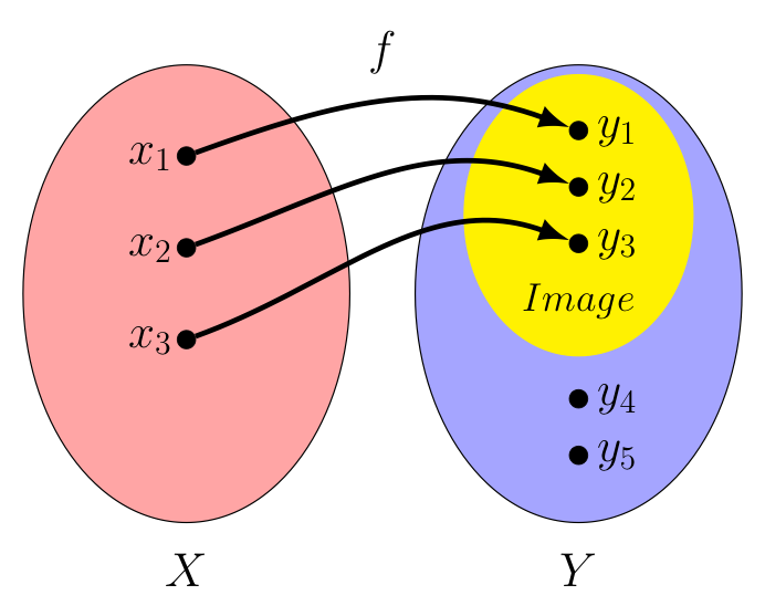
The observent reader will notice that we have carefully avoided any use of the word "range" in our discussion of the outputs associated with a function. Its absence may concern some students who have previously learned this term. Historically, the word "range" has sometimes been used to describe the co-domain of a function, and at other times to describe the image of a function. Given this ambiguity, we introduced these other two (more precise) ideas first. However, from this point forward, should we use the term range, we will mean it to be synonomous with the term "image" -- in keeping with what it represents in most calculus courses.
As one last thought related to this, one might wonder how the outputs of a function ever got associated with the term "image". While the author is unable to speak to its actual origin, he is reminded of how one can change a small drawing (an input) into a larger image (an output) by tracing where each point of the small drawing should go in the larger image with a pantograph (a physical function, in a certain sense):
Not to spoil anything, but we will have a lot more to say about this particular means of visualizing outputs of certain functions later!

Those that study English might interpret the creation of functions as an act of nominalization, which happens when creating a noun out of a verb. Consider the act of running (a noun built from the verb run) and then note how $f(x) = x^2$ similarly names the act of squaring.
Nouns are of course people, places or things. In this way, we can think of functions as just one more collection of things -- just like braids, permutations, numbers, etc.
Given what we've already seen in those other contexts, this then begs the question -- are there ways to combined functions to create other functions?
We will find great use for functions whose domains and co-domains are either all real numbers or some subsets of these. For the remainder of this section, let us assume $f$ and $g$ are functions where this is true.
That is to say, assume $f : X_f \rightarrow Y_f$ and $g : X_g \rightarrow Y_g$ where the domains and co-domains $X_f$, $Y_f$, $X_g$, and $Y_g$ are all sets of real values.
We can combine these particular types of functions to create new ones in some very straight-forward ways. However, before considering these, the following abbreviation will make writing the domains of the resulting functions a bit easier:
The set of all elements in both sets $S_1$ and $S_2$ is called the intersection of these sets, denoted by $S_1 \cap S_2$.
As a first combination to consider, let us define the product of such functions $f$ and $g$, denoted $(f \cdot g)$, as the function described by:
$$\boxed{\textrm{$(f \cdot g) : (X_f \cap X_g) \rightarrow {\mathbb R}$ with $(f \cdot g)(x) = f(x) \cdot g(x)$}}$$Notice how taking the intersection $X_f \cap X_g$ as the domain ensures we can actually find the values $f(x)$ and $g(x)$ before multiplying them together to produce the desired output.
We can define the sum and difference of $f$ and $g$, $(f+g)$ and $(f-g)$ respectively, in a similar way: $$\boxed{\textrm{$(f + g) : (X_f \cap X_g) \rightarrow {\mathbb R}$ with $(f+g)(x) = f(x) + g(x)$}}$$ $$\boxed{\textrm{$(f - g) : (X_f \cap X_g) \rightarrow {\mathbb R}$ with $(f-g)(x) = f(x) - g(x)$}}$$
We need to be a little careful when we define the quotient of two functions, as some denominators could be zero. Excluding elements from the domain where this happens serves as an easy fix: $$\boxed{\displaystyle{\left(\frac{f}{g}\right)} : \{ x \in X_f \cap X_g, g(x) \ne 0 \} \rightarrow {\mathbb R} \textrm{ with } \displaystyle{\left(\frac{f}{g}\right)(x) = \frac{f(x)}{g(x)}}}$$
There is another way we might combine functions, however -- one that takes direct inspiration from our previous work with braids and permutations, that we will discuss next.
We've used the word "composition" before, when we applied one permutation after another to produce a third. Could we do the same for functions? Could we define a new function by applying one function after another?
Recall, the composition $P_1 * P_2$ of permutations $P_1$ and $P_2$ only makes sense if $P_2$ can actually apply to the output of $P_1$. In the case of (finite) permutations, this meant they both involved the same number of elements. Remember, for permutations, the elements themselves are not really that important -- only their positions. In this way, permutations on $n$ elements can be thought of as functions whose domain and co-domain are both the integers from $1$ to $n$.
These functions can certainly be "composed" -- but what about other functions? ..especially ones whose domains and co-domains differ?
First, let us introduce a new symbol for compositions (since "$\cdot$" has already been used to express the "product" of functions above, and $(f * g)$ or $(fg)$ might be confused for the same).
Let us write $(f \circ g)$ to denote the composition of $f$ and $g$, where $g$ is applied first, and $f$ applied second -- so that $(f \circ g)(x) = f(g(x))$.
Importantly, notice that we just did something different with the order than we have done previously with compositions of permutations!
Remember $P_1 * P_2$ was evaluated "left-to-right" in so much as the resulting permutation was created by permuting with $P_1$ first, and then with $P_2$. This was a choice we made -- one designed to bring out the connections permutations have with braid concatenations. While many authors agree this is a natural order to write compositions of permutations, some don't. There sadly is no consensus on this.
However, $(f \circ g)$ is evaluated above in a "right-to-left" manner, with $g$ applied first, and then $f$. This is done so that we might avoid having to remember to swap the order of the functions when translating between $(f \circ g)$ and $f(g(x))$ forms. Think about it: if we wanted $f$ applied first, wouldn't we write $g(f(x))$?
Interestingly, the need to swap the order in this way stems from denoting $f$ evaluated at $x$ with $f(x)$, with the $x$ on the right. Some mathematicians use an alternate notation, $xf$ instead of $f(x)$. In this way, the composition $f(g(x))$ becomes $(xg)f$ where the first function encountered from left to right is the first function applied. This is not common in dealing with the mathematics associated with this course, however -- so we will opt to go the more traditional route.
Now, we must also consider the implications of having potentially different domains and co-domains.
Since in $(f \circ g)$, the function $g$ is applied first, the domain of this composition must be some subset of the domain of $g$ (possibly all of it).
Similarly, since in $(f \circ g)$, the function $f$ is applied last, the co-domain of this composition must be some subset of the co-domain of $f$ (again, possibly all of it).
Also, to ensure that we can calculate $f(g(x))$, we'll need to have $g(x)$ in the domain of $f$ for any $x$ in the domain of the composition.
Putting all of these considerations together leads to the following definition for the compostion $(f \circ g)$ of two functions $f : X_f \rightarrow Y_f$ and $g : X_g \rightarrow Y_g$:
$(f \circ g)$ is defined to be the function:
Upon considering the composition of functions -- which are a larger class of things to compose than just permutations -- the natural questions again arise:
Clearly, domain considerations will complicate things -- but let us consider each of these questions in turn, anyways.
Is functional composition associative?
That is to say, is it true that $(f \circ g) \circ h = f \circ (g \circ h)$?
Noting that the domains of both the left and right sides agree (with both being the set of all $x$ where $f(g(h(x))$ exists), consider the following: $$(f \circ (g \circ h))(x) = f((g \circ h)(x)) = f(g(h(x))) = (f \circ g)(h(x)) = ((f \circ g) \circ h)(x)$$
So yes, functional composition is clearly associative!
Is there some function that can serve as the "identity" function?
Here the complications of different possible domains are more prominent.
Recall that regardless of whether we were interested in the set of all braids $B$ on $n$ strands, or permutations $P$ of $n$ elements, or non-zero real values $x$, there was always an identity we could find (sometimes denoted $I$, other times $1$) where combining one of these things with the identity for those things left it unchanged -- regardless of the order in which that combination happened. For example, for non-zero real $x$, it is true that $x \cdot 1 = x = 1 \cdot x$.
Now suppose there is an identity function $I$ for all functions of the form $f : X \rightarrow Y$.
We want $(f \circ I) = (I \circ f) = f$, which implies $f(I(x)) = I(f(x)) = f(x)$.
Certainly if $I(w) = w$ for every $w$ in some reasonable domain for $I$, the above seems like it would be true. However, finding that "reasonable domain" proves problematic for some functions - especially if we require identical functions to have identical domains and co-domains, as previously stated.
For the curious: to see this, consider the following argument: Note that the co-domain of $f$ is $Y$, so the co-domain of $(I \circ f)$ must also be $Y$ as we require these functions are identical. By our earlier definition for composition however, the co-domain of $(I \circ f)$ is the co-domain of $I$, so the co-domain of $I$ is $Y$.
Also note that the domain of $f$ is $X$, so the domain of $(f \circ I)$ must be $X$ as well since these two functions are also identical. This implies $f(I(x))=f(x)$ for every $x$ in $X$, which in turn suggests that $I(x)$ exists for every $x$ in $X$. Hence, the domain of $I$ includes all $x$ in $X$. However, if $I(w) = w$ for every $w$ in its domain, then the co-domain of $I$, formerly found to be $Y$, must also include all $x$ in $X$.
Of course, for some functions $f : X \rightarrow Y$ this won't be true! It won't always be the case that every $x$ in $X$ is in $Y$. As an example, consider $f : \{0\} \rightarrow \{1\}$ with $f(0)=1$.
Okay, so we can't find an identity function the way we've defined things that will work for all functions of the form $f : X \rightarrow Y$. As an alternative in the same spirit, perhaps we might settle for finding two functions that both leave their domain elements untouched: $$I_X : X \rightarrow X \textrm{ where } I_X(x) = x$$ $$I_Y : Y \rightarrow Y \textrm{ where } I_Y(y) = y$$ Doing so would let us argue the following for all functions $f : X \rightarrow Y$: $$(f \circ I_X)(x) = f(I_X(x)) = f(x) = I_Y(f(x)) = (I_Y \circ f)(x)$$ Then, we at least have for all such functions, $$f \circ I_X = f \quad \textrm{and} \quad I_Y \circ f = f$$ Of course, when $X$ and $Y$ are the same set, $I_X$ and $I_Y$ are the same function.
The implication is this: for all functions $f : X \rightarrow X$ (where the domain and co-domain agree), there is indeed a unique identity function $I : X \rightarrow X$ with $I(x) = x$.
Given this, such functions have a special name -- they are called endofunctions. Note, the prefix endo- comes from the Greek word endon, meaning inner, inside, or internal. Appropriately then, an endofunction keeps its outputs inside its own domain.
However, for more general functions $f : X \rightarrow Y$, with $X$ and $Y$ possibly different sets, we'll have to settle for the above "left-identity" and "right-identity" functions that each works just in a single direction.
Do functions have inverses?
This is a more interesting question!
First, we'll have to modify what we mean by "inverse" a bit, given the difficulties associated with finding a single identity function for functions of the form $f : X \rightarrow Y$ as discussed in the previous section.
We still want inverses to "undo" one another, so let's say a function $f : X \rightarrow Y$ has inverse $f^{-1} : Y \rightarrow X$ when: $$f^{-1} \circ f = I_X \quad \textrm{ and } \quad f \circ f^{-1} = I_Y$$
Let's look at an example. Consider the function $f : X \rightarrow Y$ shown below. In this case, $f(x_i) = y_i$ for $i=1,2,3,\textrm{ and } 4$. Note we can define $f^{-1}$ by simply swapping the roles of the domain and co-domain (so arrows now go from the blue set to the red set, as shown).
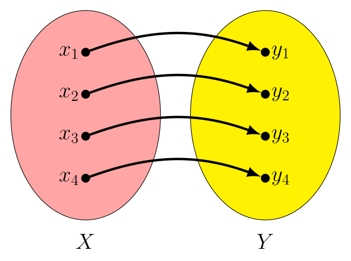
$f : X \rightarrow Y$ |
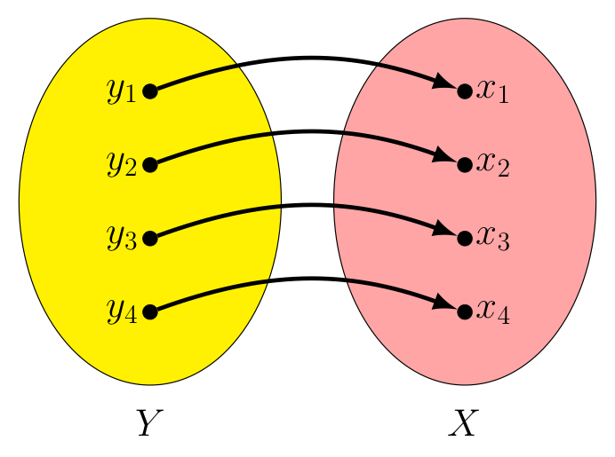
$f^{-1} : Y \rightarrow X$ |
In this way, for every $x_i$ in $X$ we have $f^{-1}(f(x_i)) = f^{-1}(y_i) = x_i$, making $f^{-1} \circ f = I_x$.
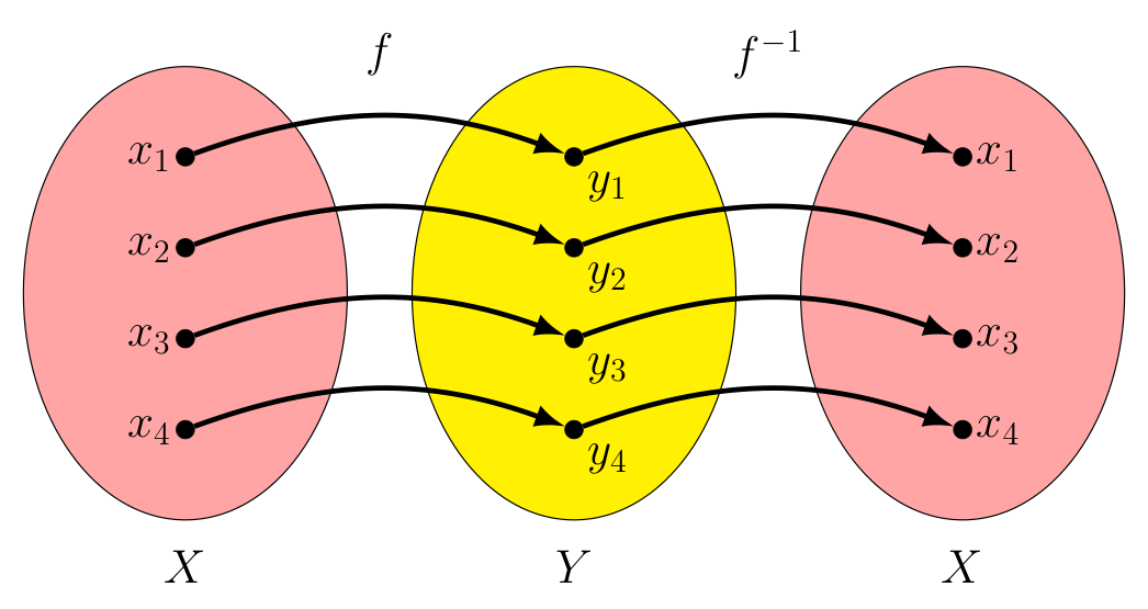
$f^{-1} \circ f$ |
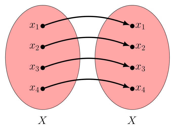
$I_X$ |
Likewise, for every $y_i$ in $Y$ we have $f(f^{-1}(y_i)) = f(x_i) = y_i$, making $f \circ f^{-1} = I_Y$.
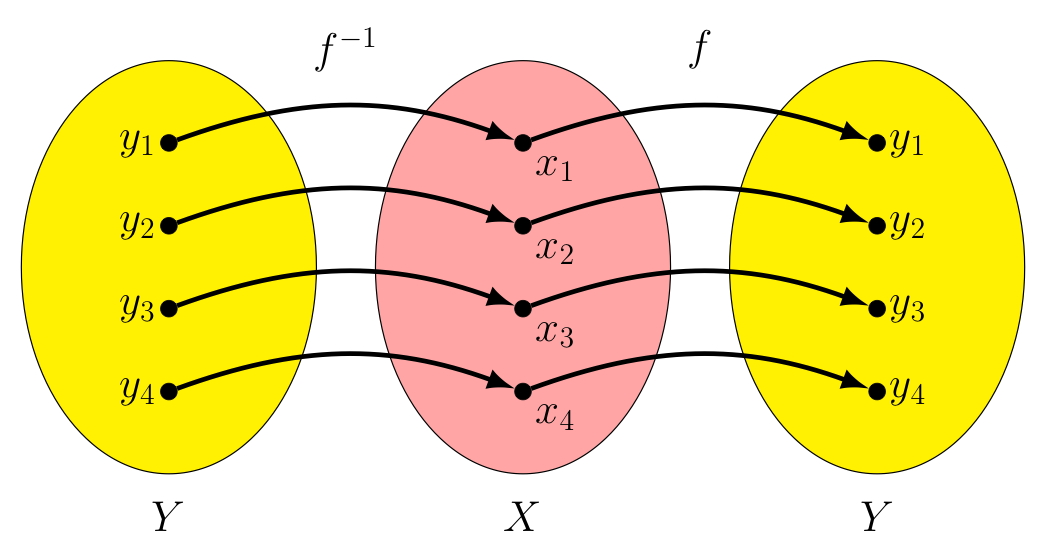
$f \circ f^{-1}$ |
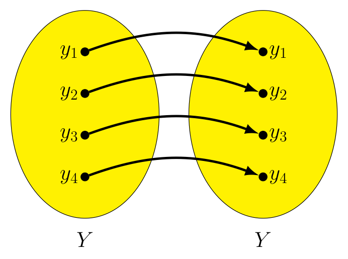
$I_Y$ |
Unfortunately, this process for finding an inverse of a given function won't always work! Suppose there are elements in the co-domain of the function that are not in its image. A simple example is shown below.
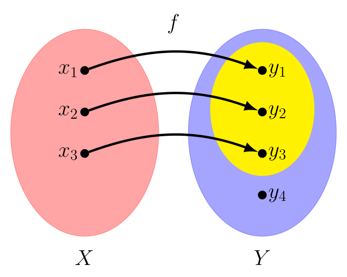
If we try to reverse things to create a function $f^{-1} : Y \rightarrow X$, realize we must define $f^{-1}(y_4)$ to be something -- but there is no value that makes sense here -- there is no $x$ in $X$ where $f(x) = y_4$!
There are similar values that prevent us from creating an inverse every time a function's image fails to cover the entirety of its domain. So, for a function to have an inverse its co-domain and image must be the same set. To give this some verbiage, we say a function with this property is surjective.
‡Note that "sur" in French means "on" (as in "on top of") and "ject" in Latin means "throw" (think of the English word "eject"). So "surjective" literally means the function throws its image (drawn yellow above) on top of the co-domain (in blue, when not covered up by the image). As a nice detail, notice how the arrows -- which traditionally are drawn so they slightly arc upwards -- are suggestive of a trajectory they might take upon being "thrown".
Equivalently, we can say $f : X \rightarrow Y$ is surjective when for every $y$ in $Y$, there is an $x$ in $X$ such that $y=f(x)$.
However, for a given function $f$ to not be surjective is not the only way for $f^{-1}$ to fail to exist! Consider the example below.
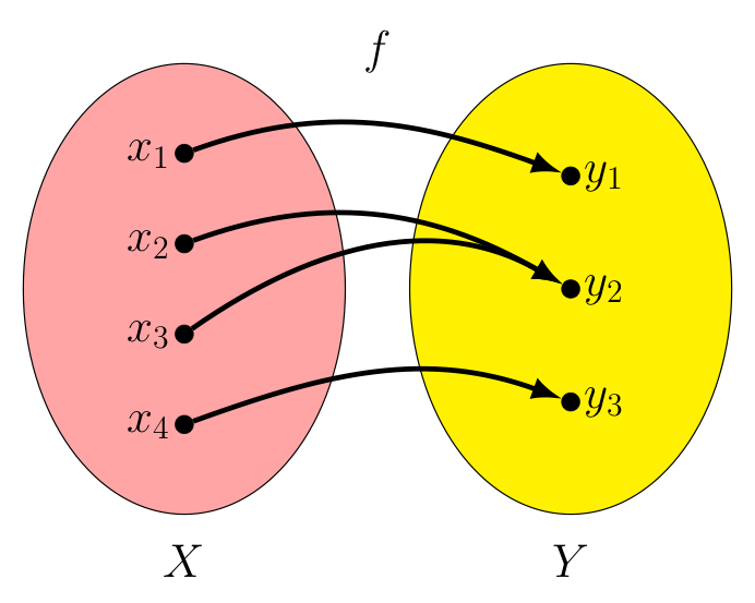
Here, we have two different inputs that result in the same output, $f(x_2) = y_2$ and $f(x_3) = y_2$.
This $f$ is still a well-defined function, of course -- such things happen all the time. Consider the function $g : {\mathbb R} \rightarrow {\mathbb R}$ that squares its inputs (i.e., $g(x) = x^2$), and note both $g(-3)=9$ and $g(3) = 9$.

as photographed by Annie Leibovitz
Well, at some point the picture at right was the last picture she had taken of Patrick Stewart AND the last picture she had taken of Ian McKellen -- two different inputs with the same output.
However, attempting to "reverse the arrows" to create an inverse for such functions will clearly run into problems!
Note, $f^{-1}$, being a function itself, must only have one output for any given input. If $f^{-1}(y_2) = x_2$, then $(f^{-1} \circ f)(x_3) \ne x_3$. Likewise, if $f^{-1}(y_2) = x_3$, then $(f^{-1} \circ f)(x_2) \ne x_2$. In both cases, we then have $(f^{-1} \circ f) \ne I_X$, which can't be!
So for a function $f : X \rightarrow Y$ to have an inverse, we also require that for any $y$ in $Y$, there is no more than one $x$ in $X$ with $y=f(x)$. Functions with this property are said to be injective.
In contrast with our earlier comment that the "sur" in "surjective" meant "on top of", here the "in" in "injective" means the same thing "in" means in English (i.e., "within"). Perhaps we think of such a function in the sense of a flow of traffic where everybody "stays within their lanes"?
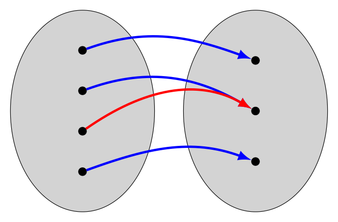
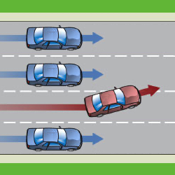
Fortunately, having a function be both surjective and injective (which we call a bijective function, or alternatively a bijection) is sufficient to ensure an inverse for that function exists.
We have seen several drawings above encouraging us to think a function as something which "throws" inputs from one set into some other set. However, when the sets involve more than a handful of elements, such drawings can easily become cumbersome -- or even impossible -- to draw.
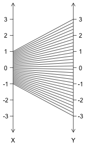
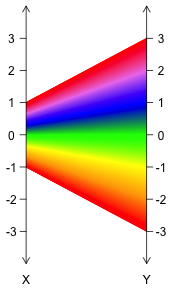
Consider the function $f : [-1,1] \rightarrow {\mathbb R}$ with $f(x) = 3x$, shown below. We omit the two ovals drawn previously to surround the elements of the domain/co-domain, opting instead to draw relevant portions of two number lines where the domain/co-domain can be found. We also left off the arrowheads to keep the picture as clean as possible -- context tells us we should think of domain elements on the left going to co-domain elements on the right.
Given the infinitude of real values in the domain, we have a couple of options. We could settle (as we do on the left) for drawing only a few representative lines connecting inputs to outputs -- although this leaves gaps, making it harder to determine the exact domain and image just from the picture. Another option (shown on the right) would be to pack the lines in tight enough to avoid gaps, but then make each line a different color so we can still track input/output pairs. The resulting "gradient effect" is certainly pretty -- but requires a lot of computation and some colored pencils (or better, some technology) to accomplish.
In truth, a compromise between these two strategies might be best. In some cases, such as with the function $f : [-2,2] \rightarrow {\mathbb R}$ with $f(x) = x^2-1$ as seen below, the lines will need to cross. Having gaps between them will help us see all the lines present (especially if some cross others), while the use of color helps us better see what input is paired with what output.
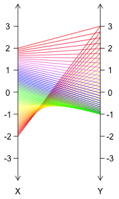
Convincing oneself that the above image does indeed represent $f(x) = x^2-1$ applied to $[-2,2]$ is fairly easy -- notice how as the input slowly moves from $-2$ to $2$, the output starts at $3$, descends to $-1$, and then ascends back to $3$. We can also immediately tell the function is not injective, given that many outputs (all but $-1$) have two lines attached them.
Still, such drawings (which are called mapping diagrams, or alternatively transformation figures) can quickly get out of hand -- making it very difficult to "see" what the function is actually doing. Consider the following image for $f : [-2,2] \rightarrow {\mathbb R}$ with $f(x) = x^4 - 3x^2 - 1$:
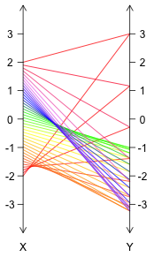
Note how in the above, as the input moves from $-2$ to $2$ the output starts at $3$, relatively rapidly descends (given the spacing of the lines) to just below $-3$, then ascends back to $-1$, followed by another fall down again below $-3$, before finally rising back to $3$. A veritable "roller-coaster"!
Hmmm... that last comment about a roller-coaster -- that could prove useful!
Thinking of how looking at a roller-coaster track, it is easy to see the different heights the roller-coaster car will take over time -- what if we re-imagined the way we visualized this function in a similar way?
With this in mind, let us first draw a horizontal number line that contains our real-valued inputs $X$ (calling this the $x$-axis). Then, for each $x$ in $X$ we mark how "high" the corresponding output $f(x)$ would be. We can draw another number line vertically to both represent our co-domain and to allow for easy comparisons between heights/outputs for different inputs. We call this vertical number line the $y$-axis.
The following gives a first-pass at such a representation. In it, we have marked the points corresponding to the specific input/output pairs considered in our previous image, and then connected these with a curve showing where other input/output pairs would be. Notice how much simpler the image for this function looks when drawn in this way! Note also how the steepness of the curve corresponds to how "spread out" the endpoints of the lines were on the right side in the previous image.
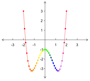
As a matter of convenient ink-saving notation, let us describe each point corresponding to some real-value input $x$ and its corresponding real-valued output $y$ with an ordered pair of coordinates, written $(x,y)$. Admittedly, this looks identical to the notation we use for an open interval (a very different thing) -- but context normally makes it quite apparent which is intended.
In case you are curious, the individual coordinates have names too! The first coordinate ($x$ above) is called the abscissa (from the Latin "linea abscissa" which means "a line cut off") and the second ($y$ above) is called the ordinate (similarly from the Latin "linea ordinata applicata", which means "line applied parallel").
As there are two real numbers in each such ordered pair, we denote the set of all such ordered pairs by ${\mathbb R}^2$ and call the plane in which the corresponding points reside the coordinate plane.
It's interesting that in the above example, all of the points corresponding to input/output pairs ended up on a single continuous curve above, don't you think? This happens a lot -- but not always. Can you describe a function where this is not true? Are there functions with domain $\mathbb R$, that nowhere along their domain can they be drawn with a "continuous stroke of a pen"?
Noting the "beaded" look of the image above, but then realizing the particular selection of input/output pairs chosen could have been different (giving us different "beads", but still lying on the same curve), there is really no need to highlight most of these inital points plotted -- we care only about the larger set of points to which they belong. As such, let us tweak our image by removing most of these "beads" -- focusing more on the set of all points $(x,y)$ where $y=f(x)$.
We also don't need to use all the different colors, as identifying the output for a given input is now as easy as looking up (or down) from the input $x$ on the $x$-axis and noting the height of the point seen there. The resulting image, which we can draw for any function whose domain and co-domain are sets of real numbers, we call the graph of $f(x)$.

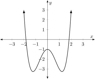
Note, we do leave two "beads" in the graph above -- at the endpoints of the curve. These are to highlight the fact that the curve does actually "stop" on the left and right sides, as drawn. If the domain had been all real values instead of $[-2,2]$, the function would have continued its ascent on both the left and the right -- which we could indicate by placing arrows at the endpoints of the curve instead, as shown below.
The earlier method for visualizing a "reals-to-reals" function, which we called mapping diagrams and/or transformation figures -- despite their potential for complexity -- certainly did make it easy to identify the domain and range/image of the function in question. Fortunately, with graphs of functions drawn in our most recently described way, this is still an easy thing to do. As an example, consider the function represented by the black curve drawn below.
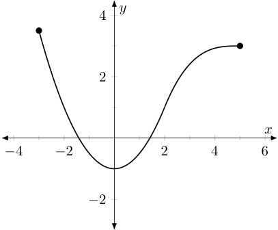
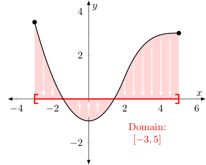
For the domain, we simply imagine all of the points of our function falling (or rising) to the $x$-axis -- the set of associated $x$-values is the domain. For the range, we do something similar, imagining all of the points of our function moving left or right until they land on the $y$-axis. The set of associated $y$-values is the range/image.
Note we don't have to ever worry about running into more than one point above or below a given input $x$ value, as if we did -- that would imply the function produced two outputs for a given input, which it can not (by definition) ever do. In this way, we say that the graphs of such functions (which take reals to reals) must always pass the vertical line test, in that any vertical line we might draw will only intersect the graph in one point (if $x$ is in the domain) or no points (if $x$ is not in the domain). As an example, the black curve below can't be described by a function $f : {\mathbb R} \rightarrow {\mathbb R}$.
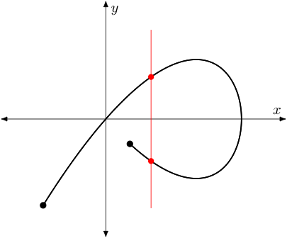
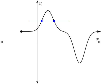
In a related way, note that we can easily detect if a function is injective too. Notice that in our earlier representation the presence of any value on the right with two (or more) lines drawn to it would be enough to know that the function was not injective. In our most recent diagram, we know a function is not injective if we can find any two points (or more) that are at the same height.
As two points at the same height would determine a horizontal line, this leads to the horizontal line test, which says if any horizontal line intersects the graph of a function (which again takes reals to reals) more than once, the function is not invertible. That is to say, it has no inverse function (since it would not be injective). As an example, the function represented by the black curve below is not invertible given the blue line intersects the curve more than once (as do many other horizontal lines, for that matter).
To pick up on an earlier point, lest the last several examples make one think that every function from $\mathbb R$ to $\mathbb R$ can be represented by a curve that can be drawn with a continuous and smooth stroke of a pen -- remember this is not the case.
As an example, the below graph also represents a function. Note we have drawn in gray some "grid lines" so determining the coordinates of various points on the graph will be easier -- but these grid lines should not be considered as part of the graph.
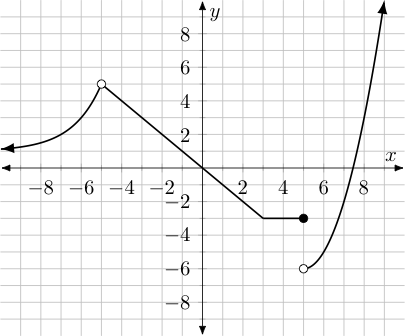
One should notice however, that there are two different types of "beads" shown: a single solid "filled-in" dot at $(5,-3)$ and two dots that are not filled at $(-5,5)$ and $(5,-6)$.
The solid black dot tells us $(5,-3)$ are the coordinates of the last point on the right where the graph is horizontal, before it "jumps" down to heights nearer to $-6$.
The other two unfilled dots highlight places where a specific $x$-value is not part of the domain. For example, the one on the left at $(-5,5)$ tells us that $x=-5$ is not included in the domain, even though $x$ values arbitrarily close to it on either side are. We say there is a "hole" in the graph at this point.
The unfilled dot on the right at $(5,-6)$ tells us something similar -- although the behavior there might better be described as a "gap" or "jump discontinuity".
Notice the function above does indeed pass the vertical line test -- even at $x=5$, a vertical line drawn there will only intersect the graph of our function at $(5,-3)$, given the hole below it. (It doesn't pass the horizontal line test, however. Alas, this function has no inverse. You win some, you lose some!)
All this aside, a significant question remains: "How do we find efficiently the graph for a given function -- like one whose formula we know?" Earlier we plotted a bunch of points and drew a curve between them. We certainly don't want to have to find the output "heights" for forty, or a hundred, or a thousand inputs, every time we need to graph a single function, right?
Even worse, if we do take the time to find all those points -- should we blindly trust that the graph of the function is a single continuous curve of some sort, and consequently just "connect the dots" from left to right?
Interestingly, this rather naive approach to graphing functions (i.e., find outputs for a whole bunch of inputs/output pairs, plot the corresponding points, and then "connect the dots") is exactly how most graphing calculators graph functions.
Not surprisingly, when there are interesting things happening between inputs where the function has been evaluated -- the calculator misses them!
For example, try graphing y=1+(x-π)^2/(x-π). We know the domain can't include $x=\pi$ as that would create a division by zero. However, no matter how close you "zoom in" on such a graph in a calculator, most will always show the output/height at $x=\pi$ to be $1$.
The moral of the story: Don't trust your calculator! It takes shortcuts sometimes that can lead to incorrect conclusions. We will address in this course how to graph many functions by hand quickly -- even faster than using a calculator in several cases, and with all of the interesting features for those graphs identified. More techniques to do the same for more complicated functions and to identify additional "interesting features" are learned in the study of calculus.
As a guiding principle -- graphing a function by "plotting points" and "connecting the dots" should be a last resort, and one whose results should automatically come with some built-in skepticism.
In the last section, we took up graphing functions by associating input/output pairs with ordered pairs that corresponded to points on the coordinate plane.
In particular recall we said the set of all such ordered pairs was denoted by a special symbol: ${\mathbb R}^2$.
Great inspiration is not required to then wonder the following: If we talk about functions whose domain is $\mathbb R$, might we not also talk about functions whose domain is ${\mathbb R}^2$? Could we do something similar with the co-domain? Can we mix and match, taking one of these to be ${\mathbb R}$ and the other to be ${\mathbb R}^2$?
Taking things even further, we can define ordered sets of $n$ real-valued coordinates for any integer $n \ge 2$. When $n=3$ we call these ordered triples, writing $(x,y,z)$ for appropriate real values $x$, $y$, and $z$. When $n \gt 3$, we call these ordered sets of $n$ real values $n$-tuples. For any positive integer $n \ge 2$, we denote the set of all $n$-tuples with ${\mathbb R}^n$.
Of course, one then naturally wonders about functions of the form $f : {\mathbb R}^n \rightarrow {\mathbb R}^m$ for various positive integers $n$ and $m$. When a function's domain or co-domain involves ${\mathbb R}^n$ with $n \ge 2$, we call it a multivariate function.
A variety of techniques can be used to visualize multivariate functions, depending on the number of coordinates involved in the domain and co-domain (also known as the dimension for each). Let us consider two special cases:
To visualize functions with domain ${\mathbb R}^2$ and co-domain $\mathbb R$, we can take a cue from what we did above, where for every input $x$ we plotted a point directly above it at a height corresponding to its corresponding output. Except now each input takes the form $(x,y)$ and can be associated with some point in the Cartesian plane.
As such, let us imagine this "plane of inputs" laid flat on a table with the points found above these at the appropriate output heights. Just as we had some "pretty" functions where the output heights for a given interval of inputs created a continuous and smooth curve -- here, we count things as "pretty" when the output heights for a given section of the input plane create a continuous and smooth surface. Below is an example:
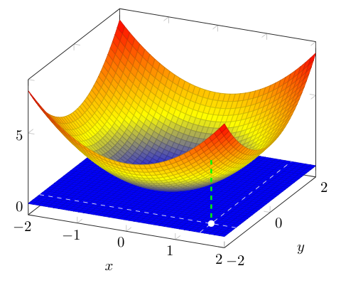
Visualizations like the one shown above are called surface plots. Note, in the plot above we have used color to make the heights of points a bit easier to follow (i.e., points at height $0$ are drawn blue -- as the height increases the color transitions first to yellow and then to red). Also, we have drawn in white one representative point in the (blue) "input plane" at $(1.5,-1.5)$, noting the point in the surface above it at a height that matches its output (follow the green dashed line).
Here, we draw inspiration from our first means for visualizing functions from $\mathbb R$ to $\mathbb R$ (i.e., transformation figures, also called mapping diagrams), where we showed what the set of inputs looked like on a number line on the left, and what the corresponding outputs looked like on a number line on the right, drawing lines taking inputs to outputs in between. The only difference is our inputs and outputs are both now two-dimensional, and we leave off the lines connecting inputs to outputs (as it would be horribly cluttered otherwise):
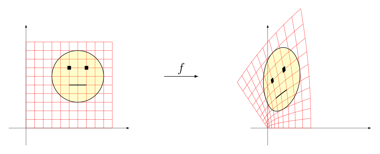
Remember the pantograph we referenced when introducing the "image" of a function? This really is a very similar idea -- except now there is much greater variety in the output images produced. They are no longer confined to scaled up or scaled down versions of the original, as produced by pantographs.