
|
A graph consists of some number of vertices and edges that connect pairs of these vertices. So any implementation of a graph must consider how to represent both of these.
As suggested by the pictures shown of graphs up to this point, representing $n$ vertices with integers $0$ through $(n-1)$ will be convenient, as doing so allows one to associate the vertices of a graph with the cells of an array. This will be advantageous in implementing many algorithms involved with graphs.
That said, these integers may not be the most natural representation of nodes. For example, a graph representing interstate routes may more naturally associate its vertices with city names. Similarly, the vertices in a graph representing a social network may be more easily associated with a person's name or (or more likely, their email address). However, we can always use a symbol table to convert between whatever the more natural representation for vertices might be given the context of the application, and the integers from $0$ to $(n-1)$ that we desire.
As for representing the edges of a graph, there are multiple options and considerations.
To decide among the choices we have, we want to think about how the graph will be used (e.g., Will we need to be able to add edges? Will we need to frequently check if there is an edge between two vertices? Will we frequently need to iterate over the vertices adjacent to a given vertex? etc...) We will want to carefully consider the implications for time and space efficiencies related to such questions for whatever edge representation we ultimately choose.
One option for representing a given graph would be to keep a list of edges in that graph. Each edge consists of two vertices, so we would need only create a linked list or array that stored pairs of vertices. The below shows how one graph (consisting of three connected components) could be represented in this way, with one edge highlighted for clarity:
| $$\require{xcolor}\begin{array}{|c|c|}\hline 0 & 1\\\hline 0 & 2\\\hline 0 & 5\\\hline 0 & 6\\\hline \color{red}{3} & \color{red}{4}\\\hline 3 & 5\\\hline 4 & 5\\\hline 4 & 6\\\hline 7 & 8\\\hline 9 & 10\\\hline 9 & 11\\\hline 9 & 12\\\hline 11 & 12\\\hline \end{array}$$ |
Let's think for a moment about the time and space efficiency of some basic actions we frequently take in relation to graphs, when using this means to represent edges. For the sake of this discussion, let us assume a graph has $V$ vertices and $E$ edges:
Adding an edge now equates to adding an element to a linked list (or to the end of an array) -- both of which are constant time operations (i.e., $\sim 1$).
Of course, if insertions are done in this extremely quick manner, we won't be able to preserve any order to our edge list as more edges are added. As a consequence, with respect to the action of determining if there is an edge between two given vertices $v$ and $w$, we will need to sequentially search the list for the pair $(v,w)$ or $(w,v)$. This, of course, is an operation that is $\sim E$.
The action of iterating over the vertices adjacent to some given vertex $v$ is likewise $\sim E$, as one needs to find every occurrence of $v$ in the list -- again accomplished through a linear search.
With regard to space efficiency, as the length of the list matches the number of edges, the space requirements also grow linearly with the number of edges added (i.e., $\sim E$).
A second option would be to represent a graph using an adjacency matrix. Essentially, one would maintain a two-dimensional $V \times V$ array boolean array adj[][], where for each edge connecting vertices $v$ and $w$, adj[v][w] == adj[w][v] == true and all other entries in the array would be false. This representation could be very naturally extended to represent digraphs, where adj[v][w] == true if and only if $v$ and $w$ were connected by an edge directed from $v$ to $w$. The below shows an example of such an adjacency matrix.
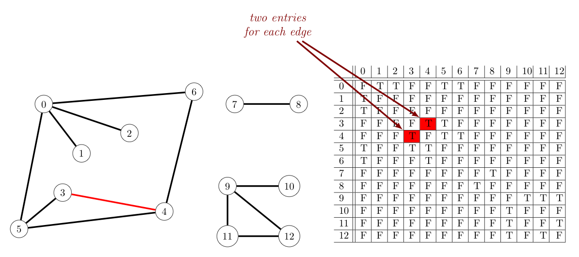
Again, let us consider some the time and space efficiencies of some basic graph operations using this representation.
Adding an edge between two vertices $u$ and $v$ with this representation is now essentially immediate (i.e., constant time $\sim 1$), as all one has to do is assign adj[u][v] the value true.
Similarly, checking if there is an edge between vertices $u$ and $v$ is as easy as checking if adj[u][v] is true or false -- so this operation is also $\sim 1$.
Iterating over the vertices adjacent to some given vertex $v$ takes a little longer, as we must sequentially inspect adj[v][1], adj[v][2], ..., keeping track of which of these values are true. As such, this operation is $\sim V$.
Where one runs into trouble is with the space analysis. As one can see, this representation for a graph requires every edge between vertices $u$ and $v$ be listed twice -- once at adj[u][v]} and another at adj[v][u]}.
However -- and far worse than duplicating edges -- the space required to store all those true/false values in a 2d array is $\sim V^2$, which will clearly be unacceptable for very large graphs.
As a further disadvantage for some contexts, this representation for graphs does not allow for parallel edges.
As a final option to consider, we could use an adjacency list to represent a graph. In this case, one would maintain a vertex-indexed array of lists -- with each list consisting of all vertices adjacent to a particular vertex. The Bag class provides a convenient way to store these lists. (Recall, a bag is essentially a stack without a pop() method, or equivalently a queue without a dequeue method.) The below provides an example:
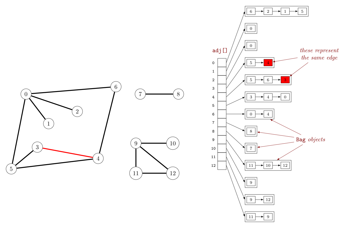
Turning our attention to the space-time complexity for this means of representing graph, let us consider again the basic graph operations examined for the previous two graph representations.
Noting that every edge shows up twice in an adjacency list representation for a graph (as suggested by the above image) -- adding an edge between vertices $v$ and $u$ is quick ($\sim 1$). One simply inserts $u$ into the bag at adj[v] and $v$ into the bag at adj[u].
Determining if there is an edge between vertices $v$ and $u$ takes a little more work. One can go immediately to the bag given by adj[v], but must then search this bag for $u$. Insisting on constant-time insertion of edges keeps us from maintaining any order to the vertices in any one bag (similar to list of edges representation), so this search must be sequential. The good news is that the maximum number of elements that must be inspected in any bag being searched is the degree of the associated vertex.
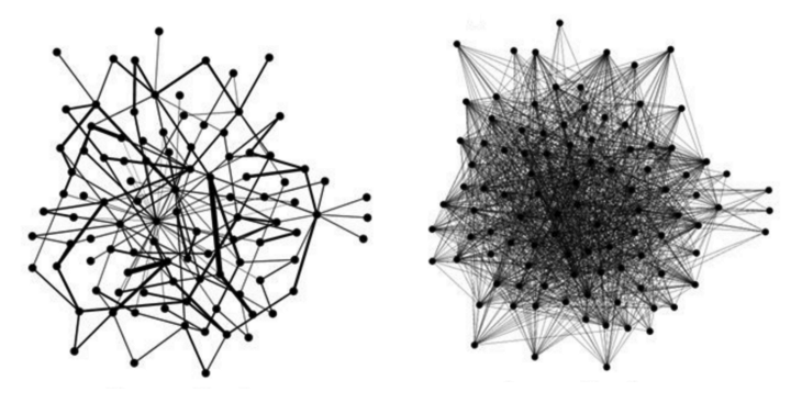
Why is this good news, you ask? Well, real-world graphs generally tend to be sparse. That is to say, while they may have a huge number of vertices, their average vertex degree is relatively small. Graphs that have a large average vertex degree relative to the number of vertices are instead called dense. An example of each is shown below.
Finally, to iterate over the vertices adjacent to a vertex $v$ is likewise proportional to the degree of $v$, as this is equivalent to iterating over the elements of the associated bag.
As for the space requirements of adjacency lists, note that we need $V$ cells in our adj[] array, and $2E$ total vertices stored in all of the bags, collectively. Thus, our space requirement is $O(E + V)$.
The following table summarizes our analysis of these three basic graph operations.
| representation | space | add edge | edge between v and w? | iterate over vertices adjacent to v |
|---|---|---|---|---|
| list of edges | $E$ | $1$ | $E$ | $E$ |
| adjacency matrix | $V^2$ | $1$* | $1$ | $V$ |
| adjacency lists | $E+V$ | $1$ | $\textrm{degree}(v)$ | $\textrm{degree}(v)$ |
As can be seen above, if we are fortunate enough to have a sparse graph (which is more often the case than not), the adjacency list wins hands down over the other two representations, and consequently are the primary means for representing graphs in practice.
Adjacency lists do have a small weakness, however. There is no way to represent parallel edges in this representation.